
4.3. Response Function or Calibration Curve
The response function for an analytical procedure is the existing relationship, within a specified range, between the response (signal, e.g., area under the curve, peak height, absorption) and the concentration (quantity) of the analyte in the sample. The calibration curve should be described preferably by a simple monotonic response function that gives accurate measurements. Note that the response function is frequently confused with the linearity criteria. However, the later criterion refers to the relationship between the quantity introduced and the quantity back-calculated from the calibration curve (see Section 4.4). Because of the confusion, it is common to see laboratory analysts try very hard to ensure that the response function is linear in the classical sense, i.e., a straight line. Not only is this not required but it is often irrelevant and can lead to large errors in measured results (e.g., for ligand binding assays). A significant source of bias and imprecision in analytical measurements can be the choice of the statistical model for the calibration curve.
4.3.1. Computational Aspects
Statistical models for calibration curves can be either linear or non-linear in their parameter(s). The choice between these two families of models will depend on the type of method and/or the range of concentrations of interest. If the range is very narrow, locally an unweighted linear model may suffice, while a larger range may require a more advanced and weighted model. High Performance Liquid Chromatography (HPLC) methods are usually linear while immunoassays are typically nonlinear. Weighting may be important for both methods because a common feature for many analytical methods is that the variance of the signal is a function of the level or quantity to be measured.
Methodologies for fitting linear and nonlinear models generally require different SAS procedures. For both model types, curves are fit by finding values for the model parameters that minimize the sum of squares of the distances between observations and the fitted curve. For linear models, parameter estimates can be derived analytically while this is not the case for many nonlinear models. Consequently, iterative procedures are often required to estimate the parameters of a nonlinear model. In this section, both linear and nonlinear models will be considered.
In case of heterogeneous variances of the signal across the concentration range, it is recommended that observations be weighted when fitting a curve. If observations are not weighted, an observation more distant to the curve than others has more influence on the curve fit. As a consequence, the curve fit may not be good where the variances are smaller. Weighting each term of the sum of squares is frequently used to solve this problem, where this can be viewed as minimizing the relative distances instead of minimizing the actual distances. When replicates are present at each concentration level, it is often better to fit the model to their average/median response values. Regardless of model type, it is assumed that all observations fit to a model are completely independent. In reality, replicates are often not independent for many analytical procedures because of the steps followed in preparation and analysis of samples. In such cases, replicates should not be used separately.
Models are typically applied on either a linear scale or log scale of the assay signal and/or the calibrator concentrations. The linear scale is used in case of homogeneous variance across the concentration range and the log scale is often more appropriate when variance increases with increasing response.
4.3.2. Linear and Polynomial Models
Most commonly used types of polynomial models include simple linear regression (with or without an intercept) and quadratic regression models.
As an illustration, consider a subset of the ELISA_CS data set (Plate A, Series 1) that includes 3 replicate measurements at each of eight concentration levels (the ELISA_CS data set is provided on the book's web site). The selected measurements are included in the CALIB data set shown below in Program 4.1. The CONCENTRATION variable is the concentration value and the rep1, rep2 and rep3 variables represent the three replicates. Program 4.1 uses the MIXED procedure to fit a linear model to the data collected in the study. The model parameters are estimated using the restricted maximum likelihood method, which is equivalent to the ordinary least square method when the data are normally distributed. The SOLUTION option requests parameter estimates which are then saved to a SAS data set specified in the ODS statement. The OUTPREDM option is used to save the predicted signal values from the fitted linear model to another SAS data set. The WEIGHT statement is used to assign weights to the individual measurements (the W variable represents the weight). For example, the weights can be defined as the inverse of the signal level or the inverse of the squared signal. In this example, the weights are defined using the following formula: w = 1/s1.3, where s is the signal level. The choice of the exponent (e.g., 1.3) depends on the relationship between the signal's variability and its average level.
Example 4-1. Fitting a simple linear regression model using PROC MIXED
data calib;
    set elisa_cs;
    if plate='A' and series=1;
    array y(3) rep1 rep2 rep3;
    do j=1 to 3;
        signal=y(j);
        w=1/signal**1.3;
    output;
    end;
proc mixed data=calib method=reml;
    model signal=concentration/solution outpredm=predict;
    weight w;
    ods output solutionf=parameter_estimates;
proc sort data=predict;
    by concentration;
axis1 minor=none label=(angle=90 'Signal') order=(0 to 4 by 1);
axis2 minor=none label=('Concentration') logbase=10 logstyle=expand;
symbol1 value=none i=join color=black line=1 width=3;
symbol2 value=dot i=none color=black height=5;
proc gplot data=predict;
    plot (pred signal)*concentration/overlay frame haxis=axis2 vaxis=axis1;
    run;
quit; |
Example. Output from Program 4.1
Solution for Fixed Effects

                                   Standard
      Effect           Estimate       Error      DF    t Value    Pr > |t|

      Intercept          0.3684     0.02850      22      12.93      <.0001
concentration 0.005802 0.000339 22 17.12 <.0001 |
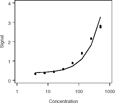
Output 4.1 lists the parameter estimates generated by PROC MIXED and associated p-values. Figure 4.1 displays the fitted regression line. It is obvious that the linear model provides a poor fit to the data.
Figure 4-1. Fit of the linear model
While Program 4.1 focuses on a simple linear regression model with an intercept, one can consider a linear regression model without an intercept, which is requested using the following MODEL statement:
model signal=concentration/solution noint;
or a quadratic regression model:
model signal=concentration concentration*concentration/solution;
In addition, the BY statement can be included in PROC MIXED to fit a calibration curve within each run.
4.3.3. Nonlinear Models (PROC NLIN)
As briefly mentioned in the introduction of this section, to fit a non-linear model, one needs to rely on iterative methods. These methods begin with an initial set of parameter values for the model of interest and update the parameter values at each step in order to improve the fit. The iterative process is stopped when the fit can no longer be improved.
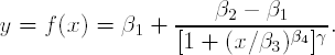
Non-linear models frequently used in curve calibration include the 4-parameter logistic regression, 5-parameter logistic regression and power model. Consider, for example, the 4-parameter logistic regression model:

where β1, β2, β3 and β4 are the top asymptote, bottom asymptote, concentration corresponding to half distance between β1 and β2, and the slope, respectively.
Both the NLIN and NLMIXED procedures can be used to fit such models. Except for the fact that they both optimize a function of interest, they do not work in the same manner. PROC NLIN fits nonlinear models by minimizing the error sum of squares and it can handle only models with fixed effects. PROC NLMIXED enables us to fit models with fixed and random effects by maximizing an approximation to the likelihood function integrated over the random effects. In this context, PROC NLMIXED is used only in models with fixed effect and thus the problem of integration is avoided.
Program 4.2 relies on PROC NLIN to model the relationship between concentration and signal levels in the subset of the ELISA_CS data set. PROC NLIN supports several iterative methods for minimizing the error sum of squares (they can be specified using the METHOD statement). The more robust methods are GAUSS, NEWTON and MARQUARDT. The default one is the GAUSS method but the most-commonly used is MARQUARDT.
Program 4.2 analyzes the CALIB data set created in Program 4.1. The initial values of the four parameters are specified in the PARAMETERS statement and the _WEIGHT_ statement is used to weight the observations when fitting the model.
Example 4-2. Fitting a 4-parameter logistic regression model using PROC NLIN
proc nlin data=calib method=marquardt outest=parameter_estimates;
    parameters top=3 bottom=0.2 c50=250 slope=1;
    model signal=top+(bottom-top)/(1+(concentration/c50)**slope);
    _weight_=w;
    output out=fitted_values predicted=pred;
proc sort data=fitted_values;
    by concentration;
axis1 minor=none label=(angle=90 'Signal') order=(0 to 4 by 1);
axis2 minor=none label=('Concentration') logbase=10 logstyle=expand;
symbol1 value=none i=join color=black line=1 width=3;
symbol2 value=dot i=none color=black height=5;
proc gplot data=fitted_values;
    plot (pred signal)*concentration/overlay frame haxis=axis2 vaxis=axis1;
    run;
quit; |
Example. Output from Program 4.2
Sum of        Mean               Approx
   Source                    DF     Squares      Square    F Value    Pr > F

   Model                      3      9.5904      3.1968    6181.88    <.0001
   Error                     20      0.0103    0.000517
   Corrected Total           23      9.6008

                                        Approx      Approximate 95% Confidence
          Parameter      Estimate    Std Error                Limits

          top              3.6611       0.1186      3.4138      3.9085
          bottom           0.3198      0.00681      0.3056      0.3340
          c50               219.9      13.9168       190.9       249.0
slope 1.2611 0.0391 1.1795 1.3427 |
Output 4.2 shows that the overall F value is very large while the standard errors of the four parameter estimates are small. This suggests that the model's fit was excellent (see also Figure 4.2). It is important to note that one sometimes encounters convergence problems and it is helpful to examine the iteration steps included in the output. If the iterative algorithm does not converge, it is prudent to explore different sets of initial values that can be obtained by a visual inspection of the raw data.
Figure 4-2. Fit of the 4-parameter logistic regression model

4.3.4. Nonlinear Models (PROC NLMIXED)
PROC NLMIXED supports a large number of iterative methods for fitting non-linear models. Unfortunately, there is no general rule for choosing the most appropriate method. The choice is problem-dependent and, most of the time, one needs to select the iterative method by trial and error (see PROC NLMIXED documentation for general recommendations).
Note that the METHOD option in PROC NLMIXED does not specify the optimization method as in PROC NLIN but rather the method for approximating the integral of the likelihood function over the random effects. The TECHNIQUE option is used in PROC NLMIXED to select the optimization method. Program 4.3 fits a 4-parameter logistic regression model to the concentration/signal data from the CALIB data set created in Program 4.1. The program uses the Newton-Raphson method with ridging as an optimization method (NRRIDG) in PROC NLMIXED. Other TECHNIQUE options include NEWRAP (Newton-Raphson optimization combining a line-search algorithm with ridging) or QUANEW (quasi-Newton). Since no random effects are included in this model, the METHOD option is not used in this example.
PROC NLMIXED does not allow to fitting of weighted regression models; however, it allows us to specify a variance function. The most popular variance function in nonlinear calibration is the power of the mean (O'Connell, Belanger and Haaland, 1993). To specify this function in Program 4.3, we introduce the VAR and THETA parameters:
model signal˜normal(expect,(expect**theta)*var);
Here VAR is the residual variance at baseline and THETA defines the rate at which this variance changes with the predicted concentration (EXPECT variable). The FITTED_VALUES data set contains the fitted value for each concentration value as well as the corresponding residual.
Example 4-3. Fitting a 4-parameter logistic regression model using PROC NLMIXED
proc nlmixed data=calib technique=nrridg;
    parms top=3 bottom=0.2 c50=250 slope=1 theta=1 var=0.0001;
    expect=top+(bottom-top)/(1+(concentration/c50)**slope);
    model signal˜normal(expect,(expect**theta)*var);
    predict top+(bottom-top)/(1+(concentration/c50)**slope) out=fitted_values;
run; |
Example. Output from Program 4.3
Parameter Estimates

                       Standard
Parameter   Estimate      Error     DF   t Value   Pr > |t|    Alpha
      Lower      Upper

top           3.6584     0.1213     24     30.16     <.0001     0.05
     3.4081     3.9087
bottom        0.3205   0.006942     24     46.18     <.0001     0.05
     0.3062     0.3349
c50           219.50    14.2383     24     15.42     <.0001     0.05
     190.12     248.89
slope         1.2628    0.04151     24     30.42     <.0001     0.05
     1.1771     1.3485
theta         1.2879     0.4150     24      3.10     0.0049     0.05
     0.4313     2.1445
var         0.000434   0.000130     24      3.35     0.0027     0.05
0.000167 0.000701 |
Output 4.3 shows that the parameter estimates and their approximate standard errors produced by PROC NLMIXED are very close to those displayed in the PROC NLIN output (Output 4.2). This is partly due to the fact that the estimated THETA parameter (1.2879) is very close to the exponent used in the weighting scheme in PROC NLIN. The fitted calibration curve is very similar to the calibration curve displayed in Figure 4.2.
4.3.5. Precision Profile for Immuno-Assays
After a calibration curve and weighting model have been chosen, a precision profile may be employed to characterize the precision of the back-calculated concentrations for unknown test samples using this calibration curve. The precision profile is a plot of the coefficient-of-variation (CV) of the calibrated concentration versus the true concentration on a log scale. Ideally, the calculated standard error of the calibrated concentration must take into account both the variability in the calibration curve and variability in the assay response. Wald's method is generally recommended for computing these standard errors (Belanger, Davidian and Giltinan, 1996) and the resulting coefficient-of-variation is given by:

where m is the number of replicates and Σ(![]() ) is the covariance matrix of the parameter estimates
) is the covariance matrix of the parameter estimates ![]() .
.
As an illustration, Program 4.4 computes a precision profile for a 5-parameter logistic model:
The γ parameter is known as the asymmetry factor and, when it is set to 1, this model is equivalent to a 4-parameter logistic model fitted in Program 4.3. In fact, Program 4.4 fits this special case of the 5-parameter logistic model by forcing the γ parameter to be 1 (note the restrictions on this parameter in the BOUNDS statement). A general 5-parameter logistic model can be obtained by removing these constraints. Further, Program 4.4 uses the IML procedure to calculate the precision profile (in general, it is easier to use the matrix language instead of DATA steps to calculate the two terms under the square root). The covariance matrix is extracted from PROC NLMIXED and is imported into PROC IML. The computed response profile is displayed in Figure 4.3.
Example 4-4. Computation of the precision profile for a 4-parameter logistic regression model using PROC NLMIXED
proc nlmixed data=calib technique=nrridg;
    parms top=3 bottom=0.2 c50=250 slope=1 theta=1 var=0.0001 g=1;
    bounds g>=1, g<=1, theta>=0, var>0; * Constraints on model parameters;
    expect=top+(bottom-top)/((1+(concentration/c50)**slope)**g);
    model signal˜normal(expect,(expect**theta)*var);
    predict top+(bottom-top)/((1+(concentration/c50)**slope)**g) out=fitted_values;
    ods output ParameterEstimates=parm_est_repl;
    ods output CovMatParmEst=cov_parm;
* Data set containing parameter estimates;
data b;
    set parm_est_repl;
    where parameter in ('top','bottom','c50','slope'),
    keep estimate;
* Data set containing the covariance matrix of the parameter estimates;
data covb;
    set cov_parm;
    where parameter in ('top','bottom','c50','slope'),
    keep top bottom c50 slope;
proc sql noprint;
    select distinct estimate into: sigma_sq from parm_est_repl where parameter='var';
    select distinct estimate into: theta from parm_est_repl where parameter='theta';
    select min(concentration) into: minconc from calib where concentration>0;
    select max(concentration) into: maxconc from calib;
    run;
    quit;
%let m=3; * Number of replicates at each concentration level;
proc iml;
    * Import the data sets;
    use b; read all into b;
    use covb; read all into covb;
    * Initialize matrices;
    y=j(101,1,0);
    h=j(101,1,0);
    hy=j(101,1,0);
    hb=j(101,4,0);
    varx0=j(101,1,0);
    pp=j(101,1,0);
    top=b[1];
    bottom=b[2];
    c50=b[3];
    slope=b[4];
* Calculate the precision profile;
do i=1 to 101;
h[i,1]=10**(log10(&minconc)+(i-1)*(log10(&maxconc)-log10(&minconc))/100);
y[i,1]=top+(bottom-top)/(1+(h[i,1]/c50)**slope);
hy[i,1]=h[i,1]*(top-bottom)/(slope*(bottom-y[i,1])*(y[i,1]-top));
hb[i,1]=h[i,1]/(slope*(y[i,1]-top));
hb[i,2]=h[i,1]/(slope*(bottom-y[i,1]));
hb[i,3]=h[i,1]/c50;
hb[i,4]=-h[i,1]*log((bottom-y[i,1])/(y[i,1]-top))/(slope**2);
varx0[i,1]=((hy[i,1]**2)*&sigma_sq*(y[i,1]**
(2*&theta))/&m)+hb[i,]*covb*hb[i,]`;
pp[i,1]=100*sqrt(varx0[i,1])/h[i,1];
end;
create plot var{h hy y pp};
append;
quit;
axis1 minor=none label=(angle=90 'CV (%)') order=(0 to 30 by 10);
axis2 minor=none label=('Concentration') logbase=10 logstyle=expand;
symbol1 value=none i=join color=black line=1 width=3;
proc gplot data=plot;
plot pp*h/frame haxis=axis2 vaxis=axis1 vref=20 lvref=34 href=4.2 lhref=34;
run;
quit; |
Figure 4-3. Precision profile based on a 4-parameter logistic regression model

It can be seen Figure 4.3 that, for concentration levels above 4 μM, the fitted model is a priori able to quantify with a precision better than 20% on a CV scale. Below this threshold, the variability of the back-calculated measurements explodes as expected because of the (low) asymptote effect. The precision achieves its maximum (approximately 2-3% on a CV scale) around the C50 value (220 μM).
The estimates of quantification limits from precision profiles are "optimistic" because they are based on only the calibration curve data themselves. These limits do not take into account matrix interference, cross-reactivity, operational factors, etc. However, these limits serve as a useful screening tool before beginning the pre-study validation exercise. Since the pre-study validation package encompasses several other sources of variability as well, if the quantification limits from a precision profile are not satisfactory, then almost definitely, the quantification limits derived from a rigorous pre-study validation package will not be satisfactory. In this case, it will be worth going back to the drawing board and further optimizing the assay protocol before proceeding to the pre-study validation phase.
4.3.6. Back-Calculated Quantities or Inverse Predictions
Once a calibration curve is fitted, concentrations of the samples of interest are calculated by inverting the estimated calibration function. In a pre-study validation, the calibration curves are fitted separately for each run and the validation samples are calculated using the calibration curve for the same run. The resulting data set consists of different concentration levels and, at each level, there are multiple runs and replicates within each run. Most of the time, the number of runs and the number of replicates are the same for all concentration levels. Inverse functions for widely used response functions are shown in Table 4.2.
For example, Program 4.5 calculates the concentrations of the validation samples (ELISA_VS dataset available on the book's companion Web site) from the 4-parameter logistic regression model fitted by series and by plate as described in Program 4.3.
Example 4-5. Concentration calculation based on a 4-parameter logistic regression model
data calib;
    set elisa_cs;
    array y(3) rep1 rep2 rep3;
    do j=1 to 3;
        signal=y(j);
    output;
    end;
proc datasets nolist;
    delete parm_est;
%macro calib(series, plate);
    proc nlmixed data=calib technique=nrridg;
        parms top=3 bottom=0.2 c50=250 slope=1 theta=1 var=0.0001;
        expect=top+(bottom-top)/(1+(concentration/c50)**slope);
        model signal˜normal(expect,(expect**(theta*2))*var);
        where series=&series and plate=&plate;
        ods output ParameterEstimates=parm_est_tmp;
    data parm_est_tmp;
        set parm_est_tmp;
        series=&series;
        plate=&plate;
    proc append data=parm_est_tmp base=parm_est;
        run;
%mend;
%calib(series=1, plate='A'),
%calib(series=1, plate='B'),
%calib(series=2, plate='A'),
%calib(series=2, plate='B'),
%calib(series=3, plate='A'),
%calib(series=3, plate='B'),
%calib(series=4, plate='A'),
%calib(series=4, plate='B'),
data valid;
    set elisa_vs;
    array y(3) rep1 rep2 rep3;
    do j=1 to 3;
        signal=y(j);
        output;
    end;
proc sort data=valid;
    by series plate;
proc transpose data=parm_est out=parm_est_t;
var estimate;
id parameter;
idlabel parameter;
by series plate;
data calc_conc;
merge valid parm_est_t;
by series plate;
drop _name_ theta var;
data calc_conc;
set calc_conc;
if plate='A' then run=series;
else run=series+4;
calc_conc=c50*((((bottom-top)/(signal-top))-1)**(1/slope));
run; |

|