7.3. Nonlinear Regression Models with a Continuous Response

In this section we first formulate the optimal design problem for general nonlinear regression models and then consider a popular dose-response model with a continuous response variable (four-parameter logistic, or E_max, model).

7.3.1. General Nonlinear Regression Model

Consider a general nonlinear regression model that is used in the analysis of concentration- or dose-response curves in a large number of clinical and pre-clinical studies. The model describes the relationship between a continuous response variable, Y, and design variable x (dose or concentration level):

Here y_ij's are often assumed to be independent observations with Var(y_ij|x_i;θ) = σ²(x_i), i.e., the variance of the response variable varies across doses or concentration levels. Also, x_i is the design variable that assumes values in a certain region, χ. Lastly, θ is an m-dimensional vector of unknown parameters.

When the response variable Y is normally distributed, the variance matrix of the MLE, , can be approximated by D(ξ,θ)/N, see (7.4), and the information matrix of a single observation is

where f(x,θ) is a vector of partial derivatives of the response function η(x,θ),

Now, as far as optimal experimental design is concerned, the sequence of steps that follow is exactly the same as for quantal dose-response models considered in Section 7.2:

It is recommended that sensitivity analysis is performed, i.e., steps 1 through 3 must be repeated for slightly different _s,s = 1,...,N_s, to verify robustness of the design ξ^*(); see Atkinson and Fedorov (1988).

Since we know that μ(x_i,θ) = g(x_i,θ) g^T(x_i,θ), the process of constructing D- or A-optimal designs for the general nonlinear regression model will be virtually identical to the process of finding optimal designs for quantal dose-response models (described in detail in Section 7.2). We only need to redefine the g(x,θ) function that determines the information matrix μ(x,θ) and sensitivity functions in (7.6) and (7.7) for the D- and A-optimality criteria, respectively.

7.3.2. Example 3: A Four-Parameter Logistic Model with a Continuous Response

The four-parameter logistic, or E_max, model, is used in many pharmaceutical applications, including bioassays (of which ELISA, or enzyme-linked immunosorbent assay, and cell-based assays are popular examples). See Finney (1976), Karpinski (1990), Hedayat et al (1997), Källén and Larsson (1999) for details and references.

This example comes from a study of a compound that inhibits the proliferation of bone marrow erythroleukemia cells in a cell-based assay (Downing, Fedorov and Leonov, 2001; Fedorov and Leonov, 2005). The logistic model used in the study is defined as follows:

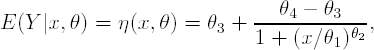
where Y is a continuous outcome variable (number of cells in the assay) and x is the design variable (concentration level). Further, θ₁ is often denoted as ED₅₀ and represents the concentration at which the median response (θ₃ + θ₄)/2 is attained, θ₂ is a slope parameter, θ₄ and θ₃ are the lower and upper asymptotes (minimal and maximal responses).

As an aside note, the four-parameter logistic model provides an example of a partially nonlinear model since θ₃ and θ₄ enter the response function in a linear fashion. This linear entry implies that the D-optimal design does not depend on values of θ₃ and θ₄ (Hill, 1980).

7.3.2.1. Computation of the D-Optimal Design

The vector of unknown parameters θ was estimated by modeling the data collected from a 96-well plate assay, with six repeated measurements at each of the ten concentrations, {500, 250, 125, ..., 500/2⁹} ng/ml, which represents a two-fold serial dilution design with N = 60 and weights w_i = 1/10. The estimated parameters are

The design region will be set to

on a log-scale. The x values will be exponentiated to compute the response function η(x,θ).

Program 7.3 constructs the D-optimal design for the introduced four-parameter logistic model by calling the %OptimalDesign1 macro. As in Programs 7.1 and 7.2, we need to define the following parameters and pass them to the macro:

• The initial design is based on ten equally-spaced and equally-weighted log-transformed concentration levels within the design region (POINTS and WEIGHTS variables).

• The grid consists of 801 equally-spaced points in χ = [−0.024,6.215].

• The true values of the model parameters are specified using the PARAMETER variable.

• The algorithm parameters are identical to those used in Programs 7.1 and 7.2.

• To specify the g(x,θ) function, we need to compute a vector of partial derivatives. The derivatives are defined in the %deriv macro. The MATRIX variable contains the values of x. The DER1, DER2, DER3 and DER4 variables represent the derivatives of the response function with respect to θ₁, θ₂, θ₃ and θ₄, respectively, and the DERIVATIVE variable contains the vector of partial derivatives.

Also, note that, in order to improve the stability of the iterative procedure, the merging constant (CMERGE) needs to be increased to 12.

As before, we will concentrate on the user-defined parameters. The complete SAS code can be found on the book's companion web site.

Example 7-3. D-optimal design for the four-parameter logistic model with a continuous response (Design parameters, algorithm parameters and g(x,θ) function)

* Design parameters;
%let points=do(-0.024,6.215,6.239/9);
%let weights=repeat(0.1,1,10);
%let grid=do(-0.024,6.215,6.239/800);
%let parameter={15.03 1.31 530 1587};
* Algorithm parameters;
%let convc=1e-9;
%let maximit=1000;
%let const1=1;
%let const2=1;
%let cmerge=12;

* G function;
%macro deriv(matrix,derivative);
    nm=nrow(&matrix);
    one=j(nm,1,1);
    dera=(parameter[4]-parameter[3])/(1+(exp(&matrix[,1])/parameter[1])
        ##parameter[2])##2#(parameter[2]/parameter[1])#(exp(&matrix[,1])
        /parameter[1])##parameter[2];
    derb=-(parameter[4]-parameter[3])/(1+(exp(&matrix[,1])/parameter[1])
        ##parameter[2])##2#(exp(&matrix[,1])/parameter[1])##parameter[2]
        #log(exp(&matrix[,1])/parameter[1]);
    derc=1-1/(1+(exp(&matrix[,1])/parameter[1])##parameter[2]);
    derd=1/(1+(exp(&matrix[,1])/parameter[1])##parameter[2]);
    &derivative=dera||derb||derc||derd;
%mend deriv;
%OptimalDesign1;

Example. Output from Program 7.3

Initial design

                                  Weight         X

                                   0.100    −0.024
                                   0.100     0.669
                                   0.100     1.362
                                   0.100     2.056
                                   0.100     2.749
                                   0.100     3.442
                                   0.100     4.135
                                   0.100     4.829
                                   0.100     5.522
                                   0.100     6.215

                                   Optimal design

                                  Weight         X

                                   0.250    −0.024
                                   0.250     2.027
                                   0.250     3.540
                                   0.250     6.215

                  Determinants of the variance-covariance matrices

                                 INITIAL     OPTIMAL

                                0.000031    0.000015

                     Variance-covariance matrix, initial design

                          COL1      COL2      COL3      COL4

                         0.019     0.000    −0.103    −0.283
                         0.000     0.000     0.027    −0.041
                        −0.103     0.027     6.745    −3.599
                        −0.283    −0.041    −3.599    12.639

Variance-covariance matrix, optimal design

                          COL1      COL2      COL3      COL4

                         0.015     0.000    −0.118    −0.181
                         0.000     0.000     0.013    −0.019
                        −0.118     0.013     5.086    −1.065
                        −0.181    −0.019    −1.065     7.087

Output 7.3 shows that the D-optimal design includes two points on the boundary of the design region (x₁^* = −0.024 and x₄^* = 6.215) and two in the middle of the design region (x₂^* = 2.027 and x₃^* = 3.540). The optimal weights are equal to 1/m = 0.25 (compare Output 7.1); see the left panel in Figure 7.5. As in Examples 1 and 2 given in Section 7.2, the sensitivity function is equal to the number of the model parameters, m = 4, at the optimal concentrations (see the right panel in Figure 7.5).

Figure 7-5. Left panel: Initial (open circles) and optimal (closed circles) designs. Right panel: Sensitivity functions for the initial (dashed curve) and optimal (solid curve) designs.

Output 7.3 also helps compare characteristics of the initial and optimal designs. The determinant of the final variance-covariance matrix is 1.5 × 10⁻⁵, compared to the value of 3.1 × 10⁻⁵ for the initial design. The variance of individual parameter estimates has improved, too. For example, the variance of θ₁ has dropped from 0.019 to 0.015. Parameter θ₁, or ED₅₀, is usually the most important for practitioners. This example illustrates a good performance of a D-optimal design with respect to other criteria of optimality, like c-criterion for the estimation of θ₁.