
2.5. Partial Least Squares for Discrimination
Perhaps the most commonly used method of statistical discrimination is simple linear discriminant analysis (LDA). A fundamental problem associated with the use of LDA in practice, however, is that the associated pooled within-groups sums-of-squares and cross-products matrix has to be invertible. For data sets with collinear features or with significantly more features than observations this may not be the case. In these situationsthere are many different options available. By far the most common in the practice of chemometrics is to first use principal components analysis (PCA) to reduce the dimension of the data, and then to follow the PCA with a version of LDA, or to simply impose an ad hoc classification rule at the level of the PCA scores and leave it at that. While both approaches are sometimes successful in identifying class structure, the dimension reduction step was not focused on the ultimate goal of discrimination.
Of course, PCA is not the only option for collinear data. Ridging or "shrinkage" can be employed to stabilize the pertinent covariance matrices so that the classical discrimination paradigms might be implemented (Friedman, 1989; Rayens, 1990; Rayens and Greene, 1991; Greene and Rayens, 1989). Alternatively, variable selection routines based in genetic algorithms are gaining popularity (e.g., Lavine, Davidson and Rayens, 2004) and have been shown to be successful in particular on microarray data. Other popular methods include flexible discriminant analysis (Ripley, 1996) and penalized discriminant analysis (Hastie et al., 1995), which are also variations on the ridging theme.
It is well known that PCA is not a particularly reliable paradigm for discrimination since it is only capable of identifying gross variability and is not capable of distinguishing "among-groups" and "within-groups" variables.Indeed, a PCA approach to discriminates the within-groups variabiliy, as often happens with chromatography studies. This point is illustrated in a small simulation study by Barker and Rayens (2003).
It turns out that partial least squares (PLS) is much more appropriate than PCA asa dimension reducing technique for the purposes of linear discrimination. Barker and Rayens fully established this connection between PLS and LDA and we will refer to their useof PLS for facilitating a discriminant analysis as PLS-LDA. Some of the details of this connection will be reviewed before illustrating how PLS-LDA can easily be implemented inSAS using the PLS procedure.
To facilitate the discussion, we will use PROC PLS to perform PLS-LDA on the same permeability data set that we used to illustrate boosting.
2.5.1. Review of PLS
PLS is based on Herman Wold's original Nonlinear Iterative Partial Least Squares (NIPALS) algorithm (Wold, 1966; Wold, 1981), adapted to reduce dimensionality in the overdetermined regression problem. However, there are many different versions of the same paradigm, some of which allow the original PLS problem to be viewed as a collection of well-posed eigenstructure problems which better facilitate PLS being connected to canonicalcovariates analysis (CCA) and, ultimately, to LDA. This is the perspective taken on PLS in this chapter. With respect to SAS, this perspective is essentially equivalent to invoking the METHOD=SIMPLS option, which we will revisit in the discussion below.
It should be noted at the outset that under this general eigenstructure perspective it is especially obvious that different sets of constraints—and whether these constraints are imposed in both the X- and Y-spaces or only one—will lead to different PLS directions. This does not seem to be well-known, or at least not often discussed in practice. With PCA the resulting "directions" or weight vectors are orthogonal and, at the same time, the associated component scores are uncorrelated. With PLS one has to choose since both uncorrelated score constraints and orthogonal weights are not simultaneously possible. Which constraint seems to be important and where you impose them depends on who you talk to. In the neurosciences, orthogonal constraints are considered essential, since the directions are often more important than the scores and having the directions be orthogonal (interpreted in practice as "independent") helps with the interpretation of the estimated "signals". Chemometricians, however, typically have no interest in an orthogonal decomposition of variable space and are much more focused on creating "new" data with uncorrelated features, which makes sense, since it is often a problem of collinearity that brings them to PLS in the first place.
For example, this latter perspective is adopted in PROC PLS, where uncorrelated score constraints are implicitly assumed. We are going to simplify our presentation by largely ignoring the constraints issue. Indeed, with all the standard constraint sets the product of the sample covariance matrix and its transpose, SxySyx, emerges at the core construct in the extraction of the PLS structure. As we will see below, it is this construct that is intimately related to Fisher's LDA. First, the definition of PLS is reviewed.
2.5.1.1. Definition of PLS
Let x and y be random p- and q-dimensional vectors with dispersion matrices Σx and Σ y, respectively (the sample matrices will be denoted by Sx and Sy). Denote the covariance of x and y by $Σxy. The first pair of PLS directions are defined as p- and q-dimensional vectors a and b that jointly maximize

The objective of the maximization in this definition can be more clearly seen by rewriting it as
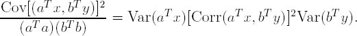
In this framework, it is easy to see how PLS can be thought of as "penalized" canonical correlations analysis (see Frank and Freidman, 1993). That is, the squared correlation term alone represents the objective of CCA. However, this objective is penalized bya variance term for the X-space and another for the Y-space. These variance terms represent the objective of principal components analysis. Hence, from this representation, PLS seeks to maximize correlation while simultaneously reducing dimension in the X- and Y-spaces.
2.5.1.2. PLS Theorem
The first PLS direction in the X-space, a1, is an eigenvector of ΣxyΣyx corresponding to the largest eigenvalue, and the corresponding first PLS direction in the Y-space, b1, is given by b1 = Σyxa1.
If orthogonality constraints are imposed on the directions in both the X- and Y-spaces, then any subsequent PLS solution, say ak+1, follows analogously, with the computation of the eigenvector of SxySyx corresponding to the (k + 1)st largest eigenvalue and the Y-space direction emerges as bk+1 = Syxak+!.If, instead of orthogonal constraints, uncorrelated score constraints are imposed, then the (k + 1)st X-space direction is an eigenvector corresponding to the largest eigenvalue of
where A(k) = [a1, a2,..., ak]p×k. There is a completely similar expression for the Y-space structure.
The described theorem is well known in the PLS literature and, for uncorrelated score constraints, a variant was first produced by de Jong (1993) when the SIMPLS procedure was introduced. Another proof of this Theorem under different constraint sets (and novel in that it does not use Lagrange multipliers) is provided in the technical report by Rayens (2000). For now, the point is simply that the derivation of the PLS directions will either directly or indirectly involve the eigenstructure of SxySyx.
In the following presentation, CCA is first connected to LDA, then, using this connection between PLS and CCA, PLS is formally connected and finally, PLS to LDA.
2.5.2. Connection between CCA and LDA
When CCA is performed on a training set, X (e.g., 71 molecular properties measured on 354 compounds described in Section 2.2) and an indicator matrix, Y, representing group membership (e.g., a 1 for a permeable compound and a 0 for a non-permeable compound), the CCA directions are just Fisher's LDA directions. This well-known fact, which was first recognized by Bartlett (1938), has been reproved more elegantly by Barker and Rayens (2003) by using the following results, which are important for this presentation.
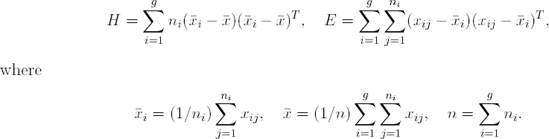
Let xij be the p-dimensional vector for the jth observation in the ith group and g be the number of groups. Denote the training set consisting of ni observations on each of p feature variables by
Let H denote the among-groups sums-of-squares and cross-products matrix and let E be the pooled within-groups sums-of-squares and cross-products matrix,
LDA, also known as "canonical discriminant analysis" (CDA) when expressed this way, manipulates the eigenstructure of E−1H. The connections between CDA and a perspective on LDA that is more focused on the minimization of misclassification probabilities are well-known andwill not be repeated here (see Kshiragar and Arseven, 1975).
There are two obvious ways that one can code the group membership in the matrix Y, either

For example, for the permeability data one could rationally choose

Note that the sample "covariance" matrix Sy is g × g and rank g − 1 while Sz is (g − 1) × (g − 1) and rank (g − 1). Regardless, the fact that both Y and Z are indicator matrices suggest that Sy and Sz will have special forms. Barker and Rayens (2003) showed the following:
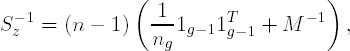
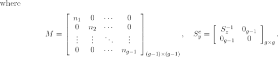
With these simple expressions for S−1z and Scy, it is possible to relate constructs that are essential to PLS-LDA to Fisher's H matrix, as will be seen in the next section.
2.5.3. Connection between PLS and LDA
Since PLS is just a penalized version of CCA and CCA is, in turn, related to LDA (Bartlett, 1938), it is reasonable to expect that PLS might have some direct connection to LDA. Barker and Rayens (2003) gave a formal statistical explanation of this connection. In particular, recall that above the USC-PLS directions were associated with the eigenstructure of SxySyx, or, for a classification application, SxzSzx, depending on how the membership matrix was coded. In either case, Barker and Rayens (2003) related the pertinent eigenstructure problem to H as follows:

It should be noted that when the Y block is coded with dummy variables, the presence of the Y-space penalty (Var(bTy)) in the definition of PLS does not seem all that appropriate, since Y-space variability is not meaningful. Barker and Rayens (2003) removed this Y-space penalty from the original objective function, reposed the PLS optimization problem and were able to show that the essential eigenstructure problem that is being manipulated in this case is one that involves exactly H, and not merely H* or H**. However, in the case of two groups, as with our permeability data, it is not hard to show that
and, hence, that the eigenstructure problems are equivalent and all proportional to (![]() 1 −
1 − ![]() )(
)(![]() 1 −
1 − ![]() )T.
)T.
The practical upshot is simple: when one uses PLS to facilitate discrimination in the "obvious" way, with the intuition of "predicting" group membership from a training set, then the attending PLS eigenstructure problem is one that depends on (essentially) Fisher's among-groups sums-of-squares and cross-products matrix H. It is, therefore, no surprise that PLS should perform better than PCA for dimension reduction when discriminant analysis on the scores is the ultimate goal. This is simply because the dimension reduction provided by PLS is determined by among-groups variability, while the dimension reduction provided by PCA is determined by total variability. It is easy to implement PLS-LDA in SAS and this is discussed next.
2.5.4. Logic of PLS-LDA
There are many rational ways that PLS can be used to facilitate discrimination. Consistent with how PCA has been used for this purpose, some will choose to simply plot the first two or three PLS-LDA "scores" and visually inspect the degree of separation, aprocess that is entirely consistent with the spirit of "territory plots" and classical CDA. The classification of an unknown may take place informally, say, by mapping it to the same two or three dimensional space occupied by the scores and then assigning it to the group that admits the closest mean score, where "closest" may be assessed in terms of Mahalanobis distance or Euclidean distance.
Alternately, the scores themselves may be viewed simply as new data that have beenappropriately "prepared" for an LDA, and a full LDA might be performed on the scores, either with misclassification rates as a goal (the DISCRIM prosedure) or visual separationand territory plots as a goal (the CANDISC procedure). Figure 2.10 helps illustrate the many options. In Section 2.5.5, we will focus on a discussion of how to produce the PLS-LDA scores with PLS procedure.
Figure 2-10. Schematic depicting the logic of PLS-LDA

2.5.5. Application
As mentioned in the Introduction, drug discovery teams often generate data that contains both descriptor information and a categorical measurement. Often, the teams desire to search for a model that can reasonably predict the response. For this section, we apply PLS-LDA to the permeability data set (the PERMY data set can be found on the book'sweb site) introduced in Section 2.2.
Recall that this data set contains 354 compounds that have been screened to assesspermeability. While the original measure of permeability was a continuous value, scientists have categorized these compounds into groups of permeable and non-permeable. In addition, this data set contains an equal number of compounds in each group. Using in-house software, 71 molecular properties, thought to be related to compound permeability, were generated for each compound and were used as the descriptors for both modeling techniques.
This is not an uncommon drug discovery-type data set—the original continuousresponse is noisy and is subsequently reduced to a binary response. Hence, we fully expect some compounds to be incorrectly classified. Also, the descriptor set is computationally derived and is over-described. With these inherent problems, many techniques would have a difficult time finding a relationship between the descriptors and the response.
2.5.5.1. Implementing PLS-LDA in SAS
The purpose of this presentation is not to detail the many options that are well known in PROC DISCRIM or PROC CANDISC, or perhaps less well known in PROC PLS; Rather this presentation is focused is focused on simply showing the reader how to use PROC PLS in conjunction with, say, PROC DISCRIM to implement PLS-LDA as described above. To betterfacilitate this discussion, we will use the permeability data, as described in the previous subsection. For this analysis, all observations are used in the training set and cross-validation is used to assess model performance.
Notice with subgroup matrices of size 177 by 71 one would not necessarily expect that any dimension reduction would be necessary and that PROC DISCRIM could be applied directly to the training set. However, many of the descriptors are physically related, so, we expect these descriptors to be correlated to some extent. In fact, each of the individual group covariance matrices, as well as the pooled covariance matrix, are 71 by 71 but only have rank 63. So, in theory, Fisher's linear discriminant analysis—whether in the form that focuses on misclassification probabilities (PROC DISCRIM) or visual among-groups separation (PROC CANDISC)—cannot be applied owing to the singularity of these matrices. Hence, these data are good candidates for first reducing dimension and then performing a formal discriminant analysis.
There is an alternative that has to be mentioned, however. When confronted with a singular covariance matrix, PROC DISCRIM will issue an innocuous warning and then proceed to construct a classification rule anyway. It is not widely known, perhaps, but in this situation SAS will employ a so-called "quasi-inverse" which is a SAS innovation. To construct the quasi-inverse "small values" are arbitrarily added to zero variance directions, thereby forcing the corresponding covariance matrices to be nonsingular and preserving the basic rationale behind the classification paradigm. Again, the purpose of this illustration is not to compare dimension reduction followed by classification with direction classification using a quasi-inverse, but it is important that the reader be aware that SAS already has one method of dealing with collinear discriminant features.
Program 2.13 performs the PLS-LDA analysis of the permeability data using PROC PLS. The initial PROC DISCRIM is invoked solely to produce the results of using the quasi-inverse. Keep in mind that the Y variable is a binary variable in this two-group case, designed to reflect corresponding group membership. In this example the first ten PLS scores (XSCR1-XSCR10) are used for the discrimination (the LV=10 option is used to request ten PLS components). For clarity of comparison, the pooled covariance matrix was used inall cases.
Example 2-13. PLS-LDA analysis of the permeability data
ods listing close;
proc discrim data=permy list crosslist noprint;
    class y;
    var x1-x71;
    run;
ods listing;
proc pls data=permy method=simpls lv=10;
    model y=x1-x71;
    output out=outpls xscore=xscr;
proc print data=outpls;
    var xscr1 xscr2;
    run;
ods listing close;
proc discrim data=outpls list crosslist noprint;
    class y;
    var xscr1-xscr10;
    run;
ods listing; |
Example. Output from Program 2.13
The PLS Procedure

                  Percent Variation Accounted for by SIMPLS Factors

              Number of
              Extracted        Model Effects        Dependent Variables
                Factors     Current       Total     Current       Total

                      1     26.6959     26.6959     18.5081     18.5081
                      2     16.6652     43.3611      2.9840     21.4921
                      3      8.3484     51.7096      3.0567     24.5488
                      4      3.5529     55.2625      3.2027     27.7515
                      5      6.2873     61.5498      0.8357     28.5872
                      6      4.0858     65.6356      0.8749     29.4621
                      7      3.5761     69.2117      0.8217     30.2838
                      8      7.0819     76.2935      0.4232     30.7070
                      9      2.2274     78.5209      0.9629     31.6699
                     10      4.7272     83.2481      0.4038     32.0737

                             Obs       xscr1      xscr2

                               1     −4.2733    −0.78608
                               2     −3.7668    −5.29011
                               3      2.0578     8.04445
                               4     −1.0728    −0.52324
                               5     −5.0157     2.37940
                               6      1.7600    −0.93071
                               7     −5.2317     3.22951
                               8     −4.2919    −6.71816
                               9     −6.3754    −3.81705
10 0.8542 −0.96708 |
Output 2.13 displays a "variance summary" produced by PROC PLS as well as a listing of first ten values of the two PLS components (XSCR1 and XSCR2). In general, navigating and understanding the PROC PLS output was discussed in great detail by Tobias (1997a, 1997b), and there is little need for us to repeat that discussion here. Rather, our purpose is, simply, to extract and then access the PLS scores for purposes of performing either a formal or ad hoc classification analysis. However, it is relevant to see how well the original feature space has been summarized by these extracted components.
When ten PLS components are requested, the "variance summary" in Output 2.13 appears for the permeability data. Notice that 26.70% of the variability in the model effects(X-space) was summarized by the first PLS component and 43.36% was summarized by the first two, etc. It may take as many as twenty components to adequately summarize the descriptor space variability. The right most columns have recorded the correlation between the X-space score and the categorical response. For a discriminant application this is not meaningful since the group coding is arbitrary.
For purposes of this chapter, the X-space scores XSCR values are what we are primarily interested in (see Figure 2.10) since it is these new data that are then transferred to PROC DISCRIM for classification. These scores appear on the PROC PLS output as shown (for two components) below. The results of the classification, summarized in terms of each group's misclassification ('error") rate, for various numbers of PLS components, are displayed in Table 2.6. These error rates are the so-called "apparent" misclassification rates and are completely standard in discriminant analysis and can be read directly off the default SAS output. Both the error ratesfor a simple reclassification of the training set (called "re-substitution" rates on theSAS output) and the leave-one-out cross-validated rates (called "cross-validated" rates on the SAS output) are reported. In all cases the pooled covariance matrix was used for the (linear) classification.
| Number of components | Re-substitution method (Cross-validation method) | |||||
|---|---|---|---|---|---|---|
| Total error rate | 0-class error rate | 1-class error rate | ||||
| PLS | PCA | PLS | PCA | PLS | PCA | |
| 2 | 0.3136 | 0.3390 | 0.2881 | 0.3220 | 0.3390 | 0.3559 |
| (0.3192) | (0.3418) | (0.2938) | (0.3277) | (0.3446) | (0.3559) | |
| 10 | 0.2345 | 0.2966 | 0.2599 | 0.2768 | 0.2090 | 0.3164 |
| (0.2514) | (0.3192) | (0.2655) | (0.2994) | (0.2373) | (0.3390) | |
| 20 | 0.2090 | 0.2885 | 0.2260 | 0.2768 | 0.1921 | 0.2881 |
| (0.2571) | (0.3390) | (0.2881) | (0.2994) | (0.2260) | (0.3785) | |
| 30 | 0.2401 | 0.2345 | 0.2260 | 0.2429 | 0.2542 | 0.2260 |
| (0.3079) | (0.2853) | (0.3051) | (0.2881) | (0.3107) | (0.2825) | |
| 40 | 0.2232 | 0.2345 | 0.2203 | 0.2712 | 0.2260 | 0.1977 |
| (0.3136) | (0.3220) | (0.3164) | (0.3616) | (0.3107) | (0.2825) | |
| 50 | 0.2429 | 0.2458 | 0.2316 | 0.2599 | 0.2542 | 0.2316 |
| (0.3333) | (0.3333) | (0.3333) | (0.3672) | (0.3333) | (0.3277) | |
| PROC DISCRIM | 0.2373 | 0.2316 | 0.2429 | |||
| with quasi-inverse | (0.3192) | (0.2938) | (0.3446) | |||
The following assessments are evident from Table 2.6:
The cross-validated estimates of total misclassification rates suggest about a 25–30% rate. This rate is fairly consistent with the non-cross-validated direct re-substitution method, although this latter method is overly optimistic, as expected.
Practically stated, the permeable and non-permeable compounds are not well separated, even with quadratic boundaries, and the corresponding misclassification rates can be expected to be fairly high in practice if one were to use the classification rule that would result from this analysis.
PROC DISCRIM with the quasi-inverse is recorded on the last line of the table. Notice that the cross-validated misclassification rates for this alternative appear to do no better, perhaps worse, than PLS-LDA.
As expected, PLS-LDA does a better job (with the exception of 30 components) than does PCA followed by an LDA. This is not really a surprise, of course, since the PLS dimension reduction step basically involved maximizing among-groups differences.
2.5.6. Summary
In Section 2.5 we have briefly reviewed the formal sense in which an empirically obvious use of PLS for the purposes of discrimination is actually optimal. This formal connection is easily turned into a functional paradigm using PROC PLS. Direct connections to the theory developed by Barker and Rayens (2003) can be had by invoking the SIMPLS option in PROC PLS, but the connections would certainly hold (on an intuitive level) for other realizations of PLS as well.
Again, what one does with the PLS scores after they are obtained seems to vary widely by user. Some will want to then perform a formal discriminant analysis (as we did in the example), while others will consider the problem "worked" at this point and simply do ad hoc classification at the level of the scores, perhaps by identifying the sample group mean score that is closest to an unknown observation.
The real point to the work of Barker and Rayens (2003) is that when classical discrimination is desired, but can't be performed owing to singular covariances (either within or pooled), then initially reducing the dimension of the problem by identifying optimal linear combinations of the original features is a rational and well-accepted approach. In fact, it is common to use PCA to accomplish this first step. One of the points madeclear by Barker and Rayens (2003) is that PLS can always be expected to do a better job at this initial reduction than can PCA. It is an open question as to whether PLS used inthis fashion would outperform SAS' use of a quasi-inverse. One of the advantages enjoyedby PLS-LDA (followed by PROC DISCRIM, perhaps) over using the quasi-inverse is that the sense in which these activities are optimal is well understood. It also would be interesting to know if employing the quasi-inverse leads to understated non-cross-validated misclassification rates in general, or if that is just a characteristic that is somehow specific to this data set. That issue is a matter for future research, however, and will not be discussed further here.