4.6. Decision Rule

It was mentioned in the Introduction that Equation (4.2), which describes the main objective of an analytical method, cannot be solved exactly. A simple way to resolve this problem and make a reliable decision, proposed by several authors (Hubert et al., 2004; Boulanger et al., 2000a, 2000b; Ho.man and Kringle, 2005), relies on computing the β-expectation tolerance intervals (Mee, 1984):

where the k factor is determined so that the expected proportion of the population falling within the interval is equal to β. If the β-expectation tolerance interval is totally included within the acceptance limits [-λ, +λ], i.e., if _M - k_M > -λ and _M + k_M < λ, the expected proportion of measurements within the same acceptance limits is greater than or equal to β. Note that the opposite statement is not true, i.e., if either _M - k_M < -λ or _M + k_M > λ, the expected proportion is not necessarily smaller than β.

Most of the time, an analytical procedure is intended to quantify over a range of quantities or concentrations. Consequently, during the validation phase, samples are prepared to adequately cover this range, and a β-expectation tolerance interval is calculated at each level.

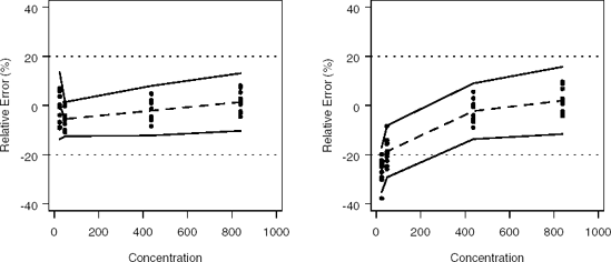
A measurement error profile is obtained, on one hand, by connecting the lower limits and, on the other hand, by connecting the upper limits. A procedure is valid over a certain range of values if the measurement error profile is included within the acceptance limits [−λ, +λ]. This concept is illustrated in Figure 4.5 for a chromatographic bio-analytical method (Hubert, 1999). In the left panel of Figure 4.5, the measurement error profile is included within the 20% acceptance limits over the entire range of concentrations, and thus the method is valid to quantify concentration values over this range. However, in the right panel of Figure 4.5, the method can only accurately quantify only concentration values greater than 300μM.

Figure 4-5. Measurement error profiles with observations, 20% acceptance limits (dotted lines), β-expectation tolerance limits (solid curves) and biases (dashed curves) expressed in terms of relative errors as a function of the concentration values for a chromatographic bio-analytical procedure

A measurement error profile gives the analyst a sense of what a procedure will be able to produce over the intended range. The interpretation of a measurement error profile is that it shows where 100β% of the measures provided by this analytical method will lie, which is directly connected to the objective of the analytical method (produce measures close to the unknown true values).

In practice, the β-expectation tolerance interval is obtained as follows (on a relative scale):

where p is the number of runs, n is the number of replicates within each run, Q_t(a,b) is the 100b% quantile of the t distribution with a degrees of freedom, and

Program 4.8 lists and plots the β-expectation tolerance limits for this study considered in Program 4.7 (the limits are included in the STAT_BY_CONC data set created by Program 4.7).

Example 4-8. Computation of the β-expectation tolerance limits

proc print data=stat_by_conc noobs split='*';
    var concentration mean low_tol_lim_rel upp_tol_lim_rel;
    run;
axis1 minor=none label=(angle=90 "Total error (%)") order=(0 to 70 by 10);
axis2 minor=none label=("Nominal concentration") logbase=10 logstyle=expand;
symbol1 value=dot i=join color=black line=1 width=3 height=3;
proc gplot data=stat_by_conc;
    format te 4.0;
    plot te*concentration/frame haxis=axis2 vaxis=axis1 vref=30 lvref=34;
    run;
    quit;
axis1 minor=none label=(angle=90 "Relative error (%)") order=(-120 to 100 by 20);
axis2 minor=none label=("Nominal concentration") logbase=10 logstyle=expand;
symbol1 value=dot i=join color=black line=1 width=3 height=3;
symbol2 value=none i=join color=black line=8 width=3;
symbol3 value=dot i=join color=black line=1 width=3 height=3;
proc gplot data=stat_by_conc;
    format low_tol_lim_rel re upp_tol_lim_rel 4.0;
    plot (low_tol_lim_rel re upp_tol_lim_rel)*concentration/overlay frame
        haxis=axis2 vaxis=axis1 vref=-30,30 lvref=34;
    run;
    quit;

Example. Output from Program 4.8

Lower 95%    Upper 95%
                 Nominal        Calculated      tolerance    tolerance
              concentration    concentration      limit        limit

                    3.5             3.2            −103         88.4
                    7.0             8.2           −37.1         70.4
                   14.1            15.5           −23.8         43.4
                   28.0            30.0            −8.1         22.7
                   56.0            57.9           −10.8         17.4
                  113.0             114           −15.0         16.9
                  225.0             235            −8.5         17.7
                  450.0             469           −12.2         20.5

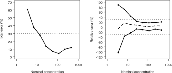
Output 4.8 shows that the tolerance interval is fully included within the 30% acceptance limits for concentration levels strictly greater than 14.1 μM. It is also important to notice that once the tolerance interval is fully included within the acceptance limits, the classical validation criteria are also satisfied. That is, the accuracy and intermediate precision are better than the usually recommended 15% threshold. Figure 4.6 provides a graphical summary of the quantities produced by Program 4.8. In the right panel of Figure 4.6, the two horizontal (dotted) lines represent the 30% acceptance limits and are equivalent to the acceptance limits in Figure 4.4 on an absolute scale. The dashed curve represents the accuracy (relative error).

Program 4.9 computes the individual total and individual relative errors and plots them along with the total error and measurement error curves displayed in Figure 4.6. The resulting total error and measurement error profiles are shown in Figure 4.7.

Figure 4-6. Total error (left panel) and measurement error (right panel) profiles

Example 4-9. Computation of individual total and individual relative errors

proc sql;
    create table te as
    select distinct 2 as type, calc_conc.concentration,
        abs(calc_conc-calc_conc.concentration)*100/calc_conc.concentration as te
    from calc_conc, stat_by_conc
    where calc_conc.concentration=stat_by_conc.concentration
    union
    select 1 as type, concentration, te from stat_by_conc;
    run;
    quit;
axis1 minor=none label=(angle=90 "Total error (%)") order=(0 to 100 by 20);
axis2 minor=none label=("Nominal concentration") logbase=10 logstyle=expand;
symbol1 value=dot i=join color=black line=1 width=3;
symbol2 value=circle i=none color=black height=5;
proc gplot data=te;
    plot te*concentration=type/vaxis=axis1 haxis=axis2 vref=30 lvref=34 nolegend;
    run;
    quit;
data me;
    set stat_by_conc;
    array y(3) low_tol_lim_rel re upp_tol_lim_rel;
    do j=1 to 3;
        me=y(j); type=j;
    output;
    end;
proc sql;
    create table me as
    select distinct 4 as type, calc_conc.concentration,
        (calc_conc-calc_conc.concentration)*100/calc_conc.concentration as me
    from calc_conc, stat_by_conc
    where calc_conc.concentration=stat_by_conc.concentration
    union
    select type, concentration, me from me;
    run;
    quit;

axis1 minor=none label=(angle=90 "Relative error (%)") order=(-120 to 100 by 20);
axis2 minor=none label=("Nominal concentration") logbase=10 logstyle=expand;
symbol1 value=dot i=join color=black line=1 width=3 height=5;
symbol2 value=none i=join color=black line=20 width=3;
symbol3 value=dot i=join color=black line=1 width=3 height=5;
symbol4 value=circle i=none color=black height=5;
proc gplot data=me;
    plot me*concentration=type/frame haxis=axis2 vaxis=axis1
 nolegend vref=-30,30 lvref=34;
    run;
    quit;

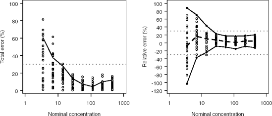
Figure 4.7 demonstrates that most of the individual relative errors are within the tolerance limits. This highlights the fact that both the total error and measurement error profiles provide clues about how extreme results may be when produced by an analytical method. That is, most results will be within the calculated limits. The measurement error profile is preferred because it is predictive (with a specified risk) of future results obtained by the method, while the total error profile is more descriptive.

Figure 4-7. Total error (left panel) and measurement error (right panel) profiles with individual total and individual relative errors

The choice of the criteria depends on the analyst's preference. If a certain amount of risk is associated with the decision, the measurement error profile should be used. Otherwise, the total error profile could be considered.

In conclusion, the measurement error profile is an easy-to-interpret tool that allows the analyst to check trueness, precision and accuracy of the method. Moreover, it is statistically meaningful and objectively oriented. Note that the lower and upper limits of quantitation can be estimated using either total error and measurement error profiles by intersecting the profiles with the acceptance limits.