
10.4. A Classical Power Analysis
Dr. Capote and his team plan their trial as follows.
Study Design
This trial follows the small (N = 62 + 62) DCA trial reported by Agbenyega et al. (2003). It will be double-blind, but instead of a 1:1 allocation, the team would like to consider giving one patient usual care only for every two patients that get QCA, where the QCA is given in a single infusion of 50 mg/kg.
Subjects
Study patients will be less than 13 years old with severe malaria complicated by lactic acidosis. "Untreatable' cases (nearly certain to die) will be excluded. These terms will require operational definitions and the CHI team will formulate the other inclusion/exclusion criteria and state them clearly in the protocol. They think it is feasible to study up to 2100 subjects in a single malaria season using just centers in Jamkatnia. If needed, they can add more centers in neighboring "Gabrieland' and increase the total size to 2700. Drop-outs should not be a problem in this study, but all studies must consider this and enlarge recruitment plans accordingly.
Primary Efficacy Outcome Measure
Death before Day 10 after beginning therapy. Almost all subjects who survive to Day 10 will have fully recovered. Time to death (i.e., survival analysis) is not a consideration.
Primary Analysis
To keep this story and example relatively simple, we will limit our attention to the basic relative risk that associates treatment group (UCO vs. QCA) with death (no or yes). For example, if 10% died under QCA and 18% died under UCO, then the estimated relative risk would be 0.10/0.18 = 0.55 in favor of QCA. p-values will be based on the likelihood ratio chi-square statistic for association in a 2 × 2 contingency table. The group's biostatistician, "Dr. Phynd Gooden," knows that the test of the treatment comparison could be made with greater power through the use of a logistic regression model that includes baseline measurements such as a severity score or lactate levels, etc. (as was done in Holloway et al., 1995). In addition, this study will be completed in a single malaria season, so performing interim analyses is not feasible. These issues are beyond the scope of this chapter.
10.4.1. Scenario for the Infinite DataSet
A prospective sample-size analysis requires the investigators to characterize the hypothetical infinite data set for their study. Too often, sample-size analysis reports fail to explain the rationale undergirding the conjectures. If we explain little or nothing, reviewers will question the depth of our thinking and planning, and thus the scientific integrity of our proposal. Be as thorough as possible and do not apologize for having to make some sound guesstimates. All experienced reviewers have had to do this themselves.
Dr. Stacpoole's N = 62 + 62 human study (Agbenyega et al., 2003) had eight deaths in each group. This yields 95% confidence intervals of [5.7%, 23.9%] for the quinine-only mortality rate (using the EXACT statement's BINOMIAL option in the FREQ procedure) and [0.40, 2.50] for the DCA relative risk (using the asymptotic RELRISK option in the OUTPUT statement in PROC FREQ). These wide intervals are of little help in specifying the scenario. However, CHI public health statistics and epidemiologic studies in the literature indicate that about 19% of these patients die within 10 days using quinine only. This figure will likely be lower for a clinical trial, because untreatable cases are being excluded and the general level of care could be much better than is typical. Finally, the Holloway et al. (1995) rat study obtained a DCA relative risk of 0.67 [95% CI: 0.44, 1.02], and the odds ratios adjusting for baseline covariates were somewhat more impressive, e.g., OR= 0.46 (one-sided p = 0.021).
Given this information, the research team conjectures that the mortality rate is 12-15% for usual care. They agree that if QCA is effective, then it is reasonable to conjecture that it will cut mortality 25-33% (relative risk of 0.67-0.75).
Topol et al. (1999) wrote about needing sufficient power to detect a clinically relevant difference between the experimental and control therapies." Some authors speak of designing studies to detect the smallest effect that is clinically relevant. How do we define such things? Everyone would agree that mortality reductions of 25-33% are clinically relevant. What about 15%? Even a 5% reduction in mortality would be considered very clinically relevant in a disease that kills so many people annually, especially because a single infusion of QCA is relatively inexpensive. Should the CHI team feel they must power this study to detect a 5% reduction in mortality? As we shall see, this is infeasible. It is usually best to ask: What do we actually know at this point? What do we think is possible? What scenarios are supportable? Will the reviewers agree with us?
10.4.2. What Allocation Ratio? One-Sided or Two-Sided Test?
Dr. Gooden is aware of the fact that the likelihood ratio chi-square test for two independent proportions can be more powerful when the sample sizes are unbalanced. Her first task is to assess how the planned 1:2 (UCO: QCA) allocation ratio affects the power. As shown in Program 10.1, this is relatively easy to do in PROC POWER. Its syntax is literal enough that we will not explain it, but note particularly the GROUPWEIGHTS statement.
Example 10-1. Compare allocation weights
* Powers at Ntotal=2100;
proc power;
    TwoSampleFreq
    GroupWeights =  (1 1) (2 3) (1 2) (1 3)  /* UCO:QCA */
    RefProportion = .15  /* Usual Care Only (UCO) mortality rate*/
    RelativeRisk =  .67   /* QCA mortality vs. UCO mortality */
    alpha = .05
    sides = 1 2
    Ntotal = 2100
    test =  lrchi
    power = .;

* Ntotal values for power = 0.90;
proc power;
    TwoSampleFreq
    GroupWeights =  (1 1) (2 3) (1 2) (1 3)/* UCO:QCA */
    RefProportion = .15  /* Usual Care Only (UCO) mortality rate*/
    RelativeRisk =  .67   /* QCA mortality vs. UCO mortality */
    alpha = .05
    sides = 1 2
    Ntotal = .
    test =  lrchi
    power = .90;
run; |
Table 10.1 displays results obtained using Program 10.1 and some simple further computations. For this conjecture of 15% mortality versus 0.67 × 15% mortality, the most efficient of these four designs is the 1:1 allocation ratio. It has a power of 0.930 or β = 0.070 with Ntotal = 2100 (α = 0.05), and to get a 0.90 power requires Ntotal = 1870. Compared to the 1:1 design, the 1:2 design has a 36% larger Type II error rate ("relative Type II risk ratio") at Ntotal = 2100 and requires 2064 subjects to achieve a 0.90 power. Thus, the 1:2 design has a relative efficiency of 1870/2064 = 0.91 and requires about 10% more subjects to achieve 0.90 power (relative inefficiency: 2064/1870 = 1.10). The relative inefficiencies for the 2:3 and 1:3 designs are 1.03 and 1.29 respectively.
| Allocation ratio (NUCO : NQCA) | |||||
|---|---|---|---|---|---|
| 1:1 | 2:3 | 1:2 | 1:3 | ||
| Ntotal = 2100 | Power | 0.930 | 0.923 | 0.905 | 0.855 |
| β | 0.070 | 0.077 | 0.095 | 0.145 | |
| Relative Type II risk ratio | 1.00 | 1.10 | 1.36 | 2.07 | |
| Power = 0.90 | Ntotal | 1870 | 1925 | 2064 | 2420 |
| Relative efficiency | 1.00 | 0.97 | 0.91 | 0.77 | |
| Relative inefficiency | 1.00 | 1.03 | 1.10 | 1.29 | |
Note that Dr. Gooden uses SIDES=1 2 in Program 10.1 to consider both one-sided and two-sided tests. Investigators and reviewers too often dogmatically call for two-sided tests only because they believe using one-sided tests is not trustworthy. But being good scientists, Dr. Capote's team members think carefully about this issue. Some argue that the scientific question is simply whether QCA is efficacious versus whether it is not efficacious, where "not efficacious" means that QCA has no effect on mortality or it increases mortality. This conforms to the one-sided test. For the design, scenario, and analysis being considered here, the one-sided test requires 1683 subjects versus 2064 for the two-sided test, giving the two-sided test a relative inefficiency of 1.23. At N = 2100, the Type II error rate for the one-sided test is β = 0.052, which is 45% less than the two-sided rate of β = 0.095. On the other hand, other members argue that it is important to assess whether QCA increases mortality. If it does, then the effective Type II error rate for the one-sided test is 1.00. This logic causes many to never view one-sided tests favorably under any circumstances. After considering these issues with Dr. Gooden, Dr. Capote decides to take the traditional approach and use a two-sided test.
For some endpoints, such as for rare adverse events or in trials involving rare diseases, the argument in favor of performing one-sided tests is often compelling. Suppose there is some fear that a potential new treatment for arthritis relief could increase the risk of gastrointestinal bleeding in some pre-specified at-risk subpopulation, say raising this from an incidence rate in the first 30 days from 8% to 24%, a relative risk of 3.0. A balanced two-arm trial with N = 450 + 450 subjects may be well powered for testing efficacy (arthritis relief), but suppose the at-risk group is only 20% of the population being sampled, so that only about N = 90 + 90 will be available for this planned sub-group analysis. Using α = 0.05, the likelihood ratio test for comparing two independent proportions will provide 0.847 power for the two-sided test and 0.910 power for the one-sided test. Thus, using a one-sided test cuts the Type II error rate from 0.153 to 0.090, a 41% reduction. Stated differently, using a two-sided test increases β by 70%. However, if this research aim is only concerned with detecting an increase in GI bleeding, why not use the statistical hypothesis—the one-sided version—that conforms to that aim? If using the two-sided test increases the Type II error rate by 70%, why is that more trustworthy?
For completeness, and because it takes so little time to do, Dr. Gooden also uses PROC POWER to find the approximate optimal allocation ratio. After iterating the group weights, she settles on using Program 10.2 to show that while the theoretical optimal is approximately 0.485:0.515, the balanced (0.500:0.500) design has almost the same efficiency.
Example 10-2. Find optimal allocation weights
proc power;
    TwoSampleFreq
    GroupWeights =       /* UCO : QCA */
    (.50 .50) (.49 .51) (.485  .515) (.48 .52) (.45 .55) (.33 .66)
    RefProportion = .15  /* Usual Care Only (UCO) mortality rate*/
    RelativeRisk =  .67   /* QCA mortality vs. UCO mortality */
    alpha = .05
    sides = 2
    Ntotal = .
    test =  LRchi /* likelihood ratio chi-square */
    power = .90
    nfractional;
run; |
Example. Output from Program 10.2
Fractional    Actual    Ceiling
   Index    Weight1    Weight2         N Total     Power    N Total

       1      0.500      0.500     1868.510571     0.900       1869
       2      0.490      0.510     1867.133078     0.900       1868
       3      0.485      0.515     1867.002923     0.900       1868
       4      0.480      0.520     1867.245653     0.900       1868
       5      0.450      0.550     1876.616633     0.900       1877
6 0.330 0.660 2061.667869 0.900 2062 |
Should the study use the less efficient 1:2 design? After substantial debate within his team, Dr. Capote decides that the non-statistical attributes of the 1:2 design give it more practical power than the 1:1 design. First, nobody has safety concerns about giving a single dose of QCA. Second, Jamkatnian health officials and parents will prefer hearing that two out of three subjects will be treated with something that could be life-saving for some. Third, the extra cost associated with a 10% increase in the sample size is not prohibitive. Given that this study's set-up costs are high and the costs associated with data analysis and reporting are unaffected by the sample size, the total cost will only increase about 3%.
10.4.3. Obtaining and Tabling the Powers
The stage is now set to carry out and report the power analysis. Please examine Program 10.3 together with Output 10.3, which contains the essential part of the results. In SAS 9.1, PROC POWER provides plain graphical displays of the results (not shown here), but lacks corresponding table displays. As this chapter was going to press, a general-purpose SAS macro, %Powtable, was being developed to help meet this need; see the book's website. Here, Dr. Gooden uses the ODS OUTPUT command and the TABULATE procedure to create a basic table.
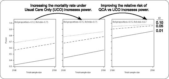
Figure 10-3. Plots for the mortality analysis showing how changing the reference proportion or the relative risk rate affects power.
Example 10-3. Power analysis for comparing mortality rates
options ls=80 nocenter FORMCHAR="|----|+|---+=|-/<>*";

proc power;
    ODS output output=MortalityPowers;
    TwoSampleFreq
    GroupWeights =  (1 2) /* 1 UCO : 2 QCA*/
    RefProportion = .12 .15 /* UCO mortality rate */
    RelativeRisk =  .75 .67  /* QCA rate vs UCO rate*/
    alpha = .01 .05 .10
    sides = 2
    Ntotal = 2100 2700
    test = LRchi  /* likelihood ratio chi-square */
    power = .;
    plot vary (panel by RefProportion RelativeRisk);

/* Avoid powers of 1.00 in table */
data MortalityPowers;
    set MortalityPowers;
    if power>0.999 then power999=0.999;
      else power999=power;

proc tabulate data=MortalityPowers format=4.3 order=data;
    format Alpha 4.3;
    class RefProportion RelativeRisk alpha NTotal;
    var Power999;
    table
    RefProportion="Usual Care Mortality"
        * RelativeRisk="QCA Relative Risk",
    alpha="Alpha"
        * Ntotal="Total N"
        * Power999=""*mean=" "/rtspace=28;
run; |
Example. Output from Program 10.3
---------------------------------------------------------- | | Alpha | | |-----------------------------| | | .010 | .050 | .100 | | |---------+---------+---------| | | Total N | Total N | Total N | | |---------+---------+---------| | |2100|2700|2100|2700|2100|2700| |--------------------------+----+----+----+----+----+----| |Usual Care |QCA Relative | | | | | | | |Mortality |Risk | | | | | | | |------------+-------------| | | | | | | |0.12 |0.75 |.329|.437|.569|.677|.687|.780| | |-------------+----+----+----+----+----+----| | |0.67 |.622|.757|.823|.905|.893|.948| |------------+-------------+----+----+----+----+----+----| |0.15 |0.75 |.438|.566|.677|.783|.781|.864| | |-------------+----+----+----+----+----+----| | |0.67 |.757|.872|.905|.960|.948|.981| ---------------------------------------------------------- |
Figure 10.3 juxtaposes three plots that were produced by using the same ODS output data set, MortalityPowers, with a SAS/GRAPH program not given here, but which is available at this book's companion Website. This shows concretely how power increases for larger UCO mortality rates or better (smaller) relative risks for QCA versus UCO.
Colleagues and reviewers should have little trouble understanding and interpreting the powers displayed as per Output 10.3. If the goal is to have 0.90 power using α = 0.05, then N = 2100 will only suffice only under the most optimistic scenario considered: that is, if the usual care mortality rate is 15% and QCA reduces that risk 33%. N = 2700 seems to be required to ensure adequate power over most of the conjecture space.
Tables like this are valuable for teaching central concepts in traditional hypothesis testing. We can see with concrete numbers how power is affected by various factors. While we can set N and α, Mother Nature sets the mortality rate for usual care and the relative risk associated with QCA efficacy.
Let us return to the phrase from Topol et al. (1997) that called for clinical trials to have adequate power "to detect a clinically relevant difference between the experimental and control therapies." With respect to our malaria study, most people would agree that even a true 5% reduction in mortality is clinically relevant and it would also be economically justifiable to provide QCA treatment given its low cost and probable safety. But could we detect such a small effect in this study? If QCA reduces mortality from 15% to 0.95 × 15% = 14.25%, then the proposed design with N = 900 + 1800 only has 0.08 power (two-sided α = 0.05). In fact, under this 1:2 design and scenario, it will require almost 104,700 patients to provide 0.90 power. This exemplifies why confirmatory trials (Phase III) are usually designed to detect plausible outcome differences that are considerably larger than "clinically relevant." The plausibility of a given scenario is based on biological principles and from data gathered in previous relevant studies of all kinds and qualities. By ordinary human nature, investigators and statisticians tend to be overly optimistic in guesstimating what Mother Nature might have set forth, and this causes our studies to be underpowered. This problem is particularly relevant when new therapies are tested against existing therapies that might be quite effective already. It is often the case that potentially small but important improvements in therapies can only be reliably assessed in very large trials. Biostatisticians are unwelcome and even sometimes disdained when they bring this news, but they did not make the Fundamental Laws of Chance—they are only charged with policing and adjudicating them.