It's important to understand exactly what the problem is here and how and when it is presented. This involves defining two things; the first being robustness as it applies to machine learning algorithms. The second, of course, is data change. Some of the content in the first part of this section is at an introductory level, but experienced data scientists may still find value in reviewing the section!

In academic terms, the robustness of a machine learning algorithm is the property that characterizes how effective your algorithm is while being applied to a dataset other than the dataset on which it was trained.

Robustness testing is a core part of machine learning methodology in any context. The importance of validation techniques such as k-fold cross-validation and the use of tests when developing models for even the simplest contexts is a consequence of machine learning algorithm vulnerability to data change.

Most datasets contain both a signal and noise. Noise may be predictable (and thus more easily managed) or it may be stochastic and difficult to treat. A dataset may contain more or less noise. Typically, datasets with more or less predictable noise are harder to train and test against the same datasets with this noise removed (which can be easily tested).

When one has trained a model on a given dataset, it is almost inevitable that this model has learned based on both the signal and noise. The concept of overfitting is generally used to describe a model that has fit so well to a given dataset that it has learned to predict based on both the signal and noise, rendering it less powerful against other samples than a model with a less exact fit.

Part of the goal of training a model is to reduce the impact of any local noise on learning as much as possible. The purpose of validation techniques that hold out a set of data to test is to ensure that any learning of noise during training happens only on noise that is local to the training set. The difference between training and test error can be used to understand the degree of overfitting between model implementations.

We've applied cross-validation in Chapter 1, Unsupervised Machine Learning. Another useful means of testing models for the overfitting is to directly add random noise in the form of jitter to the training dataset. This technique was introduced via a Kaggle notebook in October 2015 by Alexander Minushkin and offers a very interesting test. The concept is simple; by adding jitter and looking at the accuracy of prediction on the training data, we can distinguish an overfitted model (whose training error will increase more quickly as we add jitter) from a well- or poorly-fitted model:

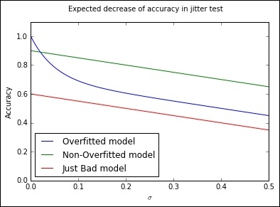
In this case, we're able to plot the results of a jitter test to easily identify whether a model has overfit. From a very strong initial position, an overfit model will typically rapidly decline in performance as small amounts of jitter are added. For better-fitting models, the loss in performance with added jitter is much reduced, with the degree of overfitting in a model being particularly obvious at low levels of added jitter (where a well-fit model will tend to outperform an overfit counterpart).

Let's look at how we implement a jitter test for overfitting. We use a familiar score, accuracy_score, defined as the proportion of class labels predicted correctly, as the basis for test scoring. Jitter is defined by simply adding random noise to the data (using np.random.normal) with the amount of noise defined by the configurable scale parameter:

from sklearn.metrics import accuracy_score

def jitter(X, scale):
    if scale > 0:        
        return X + np.random.normal(0, scale, X.shape)
    return X

def jitter_test(classifier, X, y, metric_FUNC = accuracy_score, sigmas = np.linspace(0, 0.5, 30), averaging_N = 5):
    out = []

    for s in sigmas:
        averageAccuracy = 0.0
        for x in range(averaging_N):
            averageAccuracy += metric_FUNC( y, classifier.predict(jitter(X, s)))

        out.append( averageAccuracy/averaging_N)

    return (out, sigmas, np.trapz(out, sigmas))

allJT = {}

The jitter_test itself is defined as a wrapper to normal sklearn classification, given a classifier, training data, and a set of target labels. The classifier is then called to predict against a version of the data that first has the jitter operation called against it.

At this point, we'll begin creating a number of datasets to run our jitter test over. We'll use sklearn's make_moons dataset, commonly used as a dataset to visualize clustering and classification algorithm performance. This dataset is comprised of two classes whose data points create interleaving half-circles. By adding varying amounts of noise to make_moons and using differing amounts of samples, we can create a range of example cases to run our jitter test against:

import sklearn
import sklearn.datasets

import warnings
warnings.filterwarnings("ignore", category=DeprecationWarning)

Xs = []
ys = []

#low noise, plenty of samples, should be easy
X0, y0 = sklearn.datasets.make_moons(n_samples=1000, noise=.05)
Xs.append(X0)
ys.append(y0)

#more noise, plenty of samples
X1, y1 = sklearn.datasets.make_moons(n_samples=1000, noise=.3)
Xs.append(X1)
ys.append(y1)

#less noise, few samples
X2, y2 = sklearn.datasets.make_moons(n_samples=200, noise=.05)
Xs.append(X2)
ys.append(y2)

#more noise, less samples, should be hard
X3, y3 = sklearn.datasets.make_moons(n_samples=200, noise=.3)
Xs.append(X3)
ys.append(y3)

This done, we then create a plotter object that we'll use to show our models' performance directly against the input data:

def plotter(model, X, Y, ax, npts=5000):

    xs = []
    ys = []
    cs = []
    for _ in range(npts):
        x0spr = max(X[:,0])-min(X[:,0])
        x1spr = max(X[:,1])-min(X[:,1])
        x = np.random.rand()*x0spr + min(X[:,0])
        y = np.random.rand()*x1spr + min(X[:,1])
        xs.append(x)
        ys.append(y)
        cs.append(model.predict([x,y]))
    ax.scatter(xs,ys,c=list(map(lambda x:'lightgrey' if x==0 else 'black', cs)), alpha=.35)
    ax.hold(True)
    ax.scatter(X[:,0],X[:,1],
                 c=list(map(lambda x:'r' if x else 'lime',Y)), 
                 linewidth=0,s=25,alpha=1)
    ax.set_xlim([min(X[:,0]), max(X[:,0])])
    ax.set_ylim([min(X[:,1]), max(X[:,1])])
    return

We'll use an SVM classifier as the base model for our jitter tests:

import sklearn.svm
classifier = sklearn.svm.SVC()

allJT[str(classifier)] = list()

fig, axes = plt.subplots(nrows=2, ncols=2, figsize=(11,13))
i=0
for X,y in zip(Xs,ys): 
    classifier.fit(X,y)
    plotter(classifier,X,y,ax=axes[i//2,i%2])
    allJT[str(classifier)].append (jitter_test(classifier, X, y))
    i += 1
plt.show()

The jitter test provides an effective means of assessing model overfitting and performs comparably to cross-validation; indeed, Minushkin provides evidence that it can outperform cross-validation as a tool to measure model fit quality.

Both of these tools to mitigate the overfitting work well in contexts where your algorithm is either run over data on a one-off basis or where underlying trends don't vary substantially. This is true for the majority of single-dataset problems (such as most academic or web repository datasets) or data problems where the underlying trends change slowly.

However, there are many contexts where the data involved in modeling might change over time in one or several dimensions. This can occur because of change in the methods by which data is captured, usually because new instruments or techniques come into use. For instance, video data captured by commonly-available devices has improved substantially in resolution over the decade since 2005 and the quality (and size!) of such data has increased. Whether you're using the video frames themselves or instead the file size as a parameter, you'll observe noticeable shifts in the nature, quality, and distributions of features.

Alternatively, changes in dataset variables might be caused by differences in underlying trends. The classic data schema concept of measures and dimensions comes back into play here, as we can better understand how data change is affected by considering what dimensions influence our measurement.

The key example is time. Depending on context, many variables are subject to day-of-week, month-of-year, or seasonal variations. In many cases, a helpful option might be to parameterize these variables, (as we discussed in the preceding chapter, techniques such as one-hot encoding can help our algorithms learn to parse such trends) particularly if we're dealing with periodic trends that are easily predicted (for example, the impact of month-of-year on scarf sales in a given location) and easily modeled.

A more problematic type of time series trend is non-periodic change. As in the preceding video camera example, some types of time series trends change irrevocably and in ways that might not be trivial to predict. Telemetry from software tends to be influenced by the quality and functionality of the software build live at the time the telemetry was emitted. As builds change over time, the values sent in telemetry and the variables created from those values can change radically overnight in hard-to-predict ways.

Human behavior, a hugely important factor in many datasets, helpfully changes both periodically and non-periodically. People shop more around seasonal holidays, but also change their shopping habits permanently based on new societal or technological developments.

Some of the added complexity here comes not just from the fact that single variables and their distributions are affected by time series trends, but also from how relationships between relevant factors and their associated variables will change. The relationships between variables may change in quantifiable terms. One example is how, for humans, height and weight are two variables whose relationship varies between times and locations. The BMI feature, which we might use to track this relationship, shows differing distributions when sampled across periods of time or between locations.

Furthermore, variables can change in another serious way; namely, their importance to a performant modeling algorithm may vary over time! Some variables whose values are highly relevant in some periods of time will be less relevant in others. As an example, consider how climate and weather variables affect agriculture markets. For some crops and the companies dealing in them, these variables are fairly unimportant for much of the year. At the time of crop growth and harvest, however, they become fundamentally important. To make this more complex, the strength of these factors' importance is also tied to location (and local climate).

The challenge for modeling is clear. For models that are trained once and run again on new data, managing data change can present serious challenges. For models that are dynamically recomputed based on new input data, data change can still create problems as variable distributions and relationships change and available variables become more or less valuable in generating an effective solution.

Part of the key to successfully managing data change in your application of ML is to recognize the dimensions (and there are common culprits) where change is probable and liable to affect the distributions of your features, relationships, and feature importance, which a model will attempt to pick up on.

Once you have an understanding as to what the factors in your data are that are likely to influence overfitting, you're better positioned to develop a solution that manages these factors effectively.

This said, it will still seem hugely challenging to build a single model that can resolve any potential issues. The simple response to this is that if one faces serious data change issues, the solution probably isn't to try to solve for them with a single model! In the next section, we'll be looking at ensemble methods to provide a better answer.

We've discussed a number of effective ensemble techniques that allow us to balance the twin needs for performant and robust models. However, throughout our exposition and use of these techniques, we had to decide how and when we would reduce our model's performance to improve robustness.

Indeed, a common theme in this chapter has been how to balance the conflicting objectives of creating an effective, performant model, without making this model too inflexible to respond to data change. Many of the solutions that we've seen so far have required that we trade-off one outcome against the other, which is less than ideal.

At this point, it's worth our taking a slightly wider view of our options and drawing from complimentary techniques. The need for robust, performant statistical models within evolving business landscapes is neither new nor untreated; fields such as credit risk modeling have a long history of applied statistical modeling in changing domains and have developed effective decision management methodologies in order to succeed. Data scientists can turn some of these established techniques to our own benefit via using them to help organize our own models.

One effective methodology is Champion/Challenger, a test-centric approach that involves running multiple, parallel model configurations. In addition to the model whose outputs are applied (to direct business activities or inform reporting), champion/challenger approaches training one or more alternative model configurations.

By maintaining and monitoring multiple models, one can arrange to substitute the current model as and when an alternative outperforms it. This is usually done by maintaining a performance scoring process for all models and observing the results so that a manual decision call can be made about whether and when to switch to a challenger.

While the simplest implementation may involve switching to a challenger as soon as it outperforms the main model, this is rarely done as there are risks around specific challenger models being exposed to local minima (for example, the day-of-week or month-of-year local trends). It is normal to spend a significant period assessing a challenger model, particularly ahead of sensitive applications. In complex real cases, one may even want to do additional testing by providing a sample of treatment cases to a promising challenger to determine whether it generates significant lift over the champion.

There is scope for some creativity beyond simple, "replace the challenger" succession rules. Voting-based approaches are quite common, where a top subset of the trained ensembles provides scores on a case-by-case basis and those scores treated as (weighted or unweighted) votes. Another approach involves using a Borda count, a voting system where each voter ranks the candidate solutions in order of preference. In the context of ensembling, one would typically assign each individual model's prediction a point value equal to its inverse rank (keeping each model separate!). Then one can combine these votes (usually experimenting with a range of different weightings) to generate a result.

Voting can perform fairly well with a larger number of models but is dependent on the specific modeling context and factors like the similarity of the different voters. As we discussed earlier in this chapter, it's critical to use tests such as Pearson's correlation coefficient to ensure that your model set is both performant and uncorrelated.

One may find that particular classes of input data (users, say, with specific segmentation tags) are more effectively treated by a given challenger and may implement a case routing system where multiple champions deal with different user subgroups. This approach overlaps somewhat with the benefits of boosting ensembles, but can help in production circumstances by separating concerns. However, maintaining multiple champions will increase the monitoring and oversight burden for your data team, so this option is best avoided if not entirely necessary.

A major concern to address is how we go about scoring our models, not least because there are immediate practical challenges. In particular, it is hard to compare multiple models in real contexts, given that class labels (to guide correctness) typically aren't available. In predictive contexts, this problem is compounded by the fact that the champion model's predictions are typically used to take actions that alter predicted events. This activity makes it very difficult to make assertions about how a challenger model's predictions would've performed; by taking action based on our champion's predictions, we're unable to confirm the results of our models!

The most common implementation process is to provide each challenger model with a statistically viable sample of the input data and then compare the lift from each approach. This approach inherently limits the number of challengers that one can support for some modeling problems. Another option is to leave just one statistically viable sample out of any treatment activity and use it to create a single regression test. This test is applied to the entire set of champion and challenger models, providing a meaningful basis for comparison.

The downside to this approach is that the change to a more effective model will always trail the data change by however long it takes to generate correct class labels for the test cases. While in many cases this isn't crippling (the champion model remains in place for the period it takes to generate accurate models), it can present problems in contexts where underlying conditions change rapidly compared to the training time for models.

These alternative models may simply be the next best-performing ensemble configurations; they may be older models, kept around for observation. In sophisticated operations, some challengers are configured to handle different what-if scenarios (for example, what if the temperature in this region is 2 C below expectations or what if sales are significantly below expectations). These models may have been trained on the same data as the main model or on deliberately skewed or prepared data that simulates the what-if scenario.

More challengers tend to be better (providing improved robustness and performance), provided that the challengers are not all minute variations on the same theme. Challenger models also provide a safe venue for innovation and testing, while observing effective challengers can provide useful insights into how robust your champion ensemble is likely to be to a range of possible environmental changes.

The techniques that you've learned to apply in this section have provided us with the tools to apply our existing toolkit of models to real applications in evolving environments. This chapter also discussed complications that can arise when applying ML models to production; data change, between samples or across dimensions, will cause our models to become increasingly ineffective. By thoroughly unpacking the concept of data change, we became better able to characterize this risk and recognize where and how it might present itself.

The remainder of the chapter was dedicated to techniques that provide improved model robustness. We discussed how to identify model degradation risk by looking at the underlying data and discussed some helpful heuristics to this end. We drew from existing decision management methods to learn about and use Champion/Challenger, a well-regarded process with a long history in contexts including applied machine learning. Champion/Challenger helps us organize and test multiple models in healthy competition. In conjunction with effective performance monitoring, a proactive tactical plan for model substitution will give you faster and more controllable management of the model life cycle and quality, all the while providing a wealth of valuable operational insights.