As described, in order to prevent each node from learning an unpredictable (and difficult to tune!) set of very local, free parameters, weights in a layer are shared across the entire layer. To be completely precise, the filters applied in a convolutional layer are a single set of filters, which are slid (convolved) across the input dataset. This produces a two-dimensional activation map of the input, which is referred to as the feature map.

The filter itself is subject to four hyperparameters: size, depth, stride, and zero-padding. The size of the filter is fairly self-explanatory, being the area of the filter (obviously, found by multiplying height and width; a filter need not be square!). Larger filters will tend to overlap more, and as we'll see, this can improve the accuracy of classification. Crucially, however, increasing the filter size will create increasingly large outputs. As we'll see, managing the size of outputs from convolutional layers is a huge factor in controlling the efficiency of a network.

Depth defines the number of nodes in the layer that connect to the same region of the input. The trick to understanding depth is to recognize that looking at an image (for people or networks) involves processing multiple different types of property. Anyone who has ever looked at all the image adjustment sliders in Photoshop has an idea of what this might entail. Depth is sometimes referred to as a dimension in its own right; it almost relates to the complexity of an image, not in terms of its contents but in terms of the number of channels needed to accurately describe it.

It's possible that the depth might describe color channels, with nodes mapped to recognize green, blue, or red in the input. This, incidentally, leads to a common convention where depth is set to three (particularly at the first convolution layer). It's very important to recognize that some nodes commonly learn to express less easily-described properties of input images that happen to enable a convnet to learn that image more accurately. Increasing the depth hyperparameter tends to enable nodes to encode more information about inputs, with the attendant problems and benefits that you might expect.

As a result, setting the depth parameter to too small a value tends to lead to poor results because the network doesn't have the expressive depth (in terms of channel count) required to accurately characterize input data. This is a problem analogous to not having enough features, except that it's more easily fixed; one can tune the depth of the network upward to improve the expressive depth of the convnet.

Equally, setting the depth parameter to too small a value can be redundant or harmful to performance, thereafter. If in doubt, consider testing the appropriate depth value during network configuration via hyperparameter optimization, the elbow method, or another technique.

Stride is a measure of spacing between neurons. A stride value of one will lead every element of the input (for an image, potentially every pixel) to be the center of a filter instance. This naturally leads to a high degree of overlap and very large outputs. Increasing the stride causes less of an overlap in the receptive fields and the output's size is reduced. While tuning the stride of a convnet is a question of weighing accuracy against output size, it can generally be a good idea to use smaller strides, which tend to work better. In addition, a stride value of one enables us to manage down-sampling and scale reduction at pooling layers (as we'll discuss later in the chapter).

The following diagram graphically displays both Depth and Stride:

The final hyperparameter, zero-padding, offers an interesting convenience. Zero-padding is the process of setting the outer values (the border) of each receptive field to zero, which has the effect of reducing the output size for that layer. It's possible to set one, or multiple, pixels around the border of the field to zero, which reduces the output size accordingly. There are, of course, limits; obviously, it's not a good idea to set zero-padding and stride such that areas of the input are not touched by a filter! More generally, increasing the degree of zero-padding can cause a decrease in effectiveness, which is tied to the increased difficulty of learning features via coarse coding. (Refer to the Understanding pooling layers section in this chapter.)

However, zero-padding is very helpful because it enables us to adjust the input and output sizes to be the same. This is a very common practice; using zero-padding to ensure that the size of the input layer and output layer are equal, we are able to easily manage the stride and depth values. Without using zero-padding in this way, we would need to do a lot of work tracking input sizes and managing network parameters simply to make the network function correctly. In addition, zero-padding also improves performance as, without it, a convnet will tend to gradually degrade content at the edges of the filter.

In order to calibrate the number of nodes, appropriate stride, and padding for successive layers when we define our convnet, we need to know the size of the output from the preceding layer. We can calculate the spatial size of a layer's output (O) as a function of the input image size (W), filter size (F), stride (S), and the amount of zero-padding applied (P), as follows:

If O is not an integer, the filters do not tile across the input neatly and instead extend over the edge of the input. This can cause some problematic issues when training (normally involving thrown exceptions)! By adjusting the stride value, one can find a whole-number solution for O and train effectively. It is normal for the stride to be constrained to what is possible given the other hyperparameter values and size of the input.

We've discussed the hyperparameters involved in correctly configuring the convolutional layer, but we haven't yet discussed the convolution process itself. Convolution is a mathematical operator, like addition or derivation, which is heavily used in signal processing applications and in many other contexts where its application helps simplify complex equations.

Loosely speaking, convolution is an operation over two functions, such as to produce a third function that is a modified version of one of the two original functions. In the case of convolution within a convnet, the first component is the network's input. In the case of convolution applied to images, convolution is applied in two dimensions (the width and height of the image). The input image is typically three matrices of pixels—one for each of the red, blue, and green color channels, with values ranging between 0 and 255 in each channel.

The second input to the convolution operation is the convolution kernel, a single matrix of floating point numbers that acts as a filter on the input matrices. The output of this convolution operation is the feature map. The convolution operation works by sliding the filter across the input, computing the dot product of the two arguments at each instance, which is written to the feature map. In cases where the stride of the convolutional layer is one, this operation will be performed across each pixel of the input image.

The main advantage of convolution is that it reduces the need for feature engineering. Creating and managing complex kernels and performing the highly specialized feature engineering processes needed is a demanding task, made more challenging by the fact that feature engineering processes that work well in one context can work poorly in most others. While we discuss feature engineering in detail in Chapter 7, Feature Engineering Part II, convolutional nets offer a powerful alternative.

CNN, however, incrementally improve their kernel's ability to filter a given input, thus automatically optimizing their kernel. This process is accelerated by learning multiple kernels in parallel at once. This is feature learning, which we've encountered in previous chapters. Feature learning can offer tremendous advantages in time and in increasing the accessibility of many problems. As with our earlier SDA and DBN implementations, we would look to pass our learned features to a much simpler, shallow neural network, which uses these features to classify the input image.

Stacking convolutional layers allows us to create a topology that effectively creates features as feature maps for complex, noisy input data. However, convolutional layers are not the only component of a deep network. It is common to weave convolutional layers in with pooling layers. Pooling is an operation over feature maps, where multiple feature values are aggregated into a single value—mostly using a max (max-pooling), mean (mean-pooling), or summation (sum-pooling) operation.

Pooling is a fairly natural approach that offers substantial advantages. If we do not aggregate feature maps, we tend to find ourselves with a huge amount of features. The CIFAR-10 dataset that we'll be classifying later in this chapter contains 60,000 32 x 32 pixel images. If we hypothetically learned 200 features for each image—over 8 x 8 inputs—then at each convolution, we'd find ourselves with an output vector of size (32 – 8+1) * (32 – 8+1) * 200, or 125,000 features per image. Convolution produces a huge amount of features that tend to make computation very expensive and can also introduce significant overfitting problems.

The other major advantage provided by a pooling operation is that it provides a level of robustness against the many, small deviations and variances that occur in modeling noisy, high-dimensional data. Specifically, pooling prevents the network learning the position of features too specifically (overfitting), which is obviously a critical requirement in image processing and recognition settings. With pooling, the network no longer fixates on the precise location of features in the input and gains a greater ability to generalize. This is called translation-invariance.

Max-pooling is the most commonly applied pooling operation. This is because it focuses on the most responsive features in question that should, in theory, make it the best candidate for image recognition and classification purposes. By a similar logic, min-pooling tends to be applied in cases where it is necessary to take additional steps to prevent an overly sensitive classification or overfitting from occurring.

For obvious reasons, it's prudent to begin modeling using a quickly applied and straightforward pooling method such as max-pooling. However, when seeking additional gains in network performance during later iterations, it's important to look at whether your pooling operations can be improved on. There isn't any real restriction in terms of defining your own pooling operation. Indeed, finding a more effective subsampling method or alternative aggregation can substantially improve the performance of your model.

In terms of theano code, a max-pooling implementation is pretty straightforward and may look like this:

from theano.tensor.signal import downsample

input = T.dtensor4('input')
maxpool_shape = (2, 2)
pool_out = downsample.max_pool_2d(input, maxpool_shape, ignore_border=True)
f = theano.function([input],pool_out)

The max_pool_2d function takes an n-dimensional tensor and downscaling factor, in this case, input and maxpool_shape, with the latter being a tuple of length 2, containing width and height downscaling factors for the input image. The max_pool_2d operation then performs max-pooling over the two trailing dimensions of the vector:

invals = numpy.random.RandomState(1).rand(3, 2, 5, 5)

pool_out = downsample.max_pool_2d(input, maxpool_shape, ignore_border=False)
f = theano.function([input],pool_out)

The ignore_border determines whether the border values are considered or discarded. This max-pooling operation produces the following, given that ignore_border = True:

[[ 0.72032449  0.39676747]
[ 0.6852195   0.87811744]]

As you can see, pooling is a straightforward operation that can provide dramatic results (in this case, the input was a 5 x 5 matrix, reduced to 2 x 2). However, pooling is not without critics. In particular, Geoffrey Hinton offered this pretty delightful soundbite:

This is a bold statement, but it makes sense. Hinton's telling us that the pooling operation, as an aggregation, does what any aggregation necessarily does—it reduces the data to a simpler and less informationally-rich format. This wouldn't be too damaging, except that Hinton goes further.

Even if we'd reduced the data down to single values for each pool, we could still hope that the fact that multiple pools overlap spatially would still present feature encodings. (This is the coarse coding referred to by Hinton.) This is also quite an intuitive concept. Imagine that you're listening in to a signal on a noisy radio frequency. Even if you only caught one word in three, it's probable that you'd be able to distinguish a distress signal from the shipping forecast!

However, Hinton follows up by observing that coarse coding is not as effective in learning pose (position, orientation, and scale). There are so many permutations in viewpoint relative to an object that it's unlikely two images would be alike and the sheer variety of possible poses becomes a challenge for a convolutional network using pooling. This suggests that an architecture that does not overcome this challenge may not be able to break past an upper limit for image classification.

However, the general consensus, at least for now, is that even after acknowledging all of this, it is still highly advantageous in terms of efficiency and translation-invariance to continue using pooling operations in convnets. Right now, the argument goes that it's the best we have!

Meanwhile, Hinton proposed an alternative to convnets in the form of the transforming autoencoder. The transforming autoencoder offers accuracy improvements on learning tasks that require a high level of precision (such as facial recognition), where pooling operations would cause a reduction in precision. The Further reading section of this chapter contains recommendations if you are interested in learning more about the transforming autoencoder.

So, we've spent quite a bit of time digging into the convolutional neural network—its components, how they work, and their hyperparameters. Before we move on to put the theory into action, it's worth discussing how all of these theoretical components fit together into a working architecture. To do this, let's discuss what training a convnet looks like.

The means of training a convolutional network will be familiar to readers of the preceding chapters. The convolutional architecture itself is used to pretrain a simpler network structure (for example, an MLP). The backpropagation algorithm is the standard method to compute the gradient when pretraining. During this process, every layer undertakes three tasks:

Repetition of this process allows us to achieve increasing kernel performance until we reach a point of convergence. At this point, we will hope to have developed a set of features sufficient that the capping network is able to effectively classify over these features.

This process can execute slowly, even on a fairly advanced GPU. Some recent developments have helped accelerate the training process, including the use of the Fast Fourier Transform to accelerate the convolution process (for cases where the convolution kernel is of roughly equal size to the input image).

So far, we've discussed some of the elements required to create a CNN. The next subject of discussion should be how we go about combining these components to create capable convolutional nets as well as which combinations of components can work well. We'll draw guidance from a number of forerunning convnet implementations as we build an understanding of what is commonly done as well as what is possible.

Probably the best-known convolutional network implementation is Yann LeCun's LeNet. LeNet has gone through several iterations since LeNet-1 in late 1980, but has been increasingly effective at performing tasks including handwritten digit and image classification. LeNet is structured using alternating convolution and pooling layers capped by an MLP, as follows:

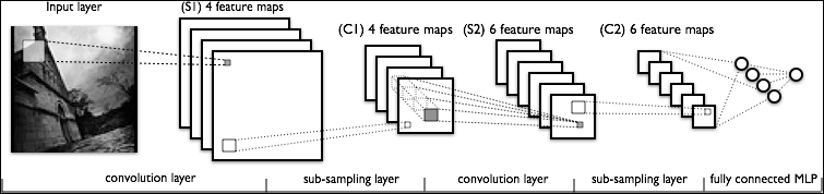
Each layer is partially-connected, as we discussed earlier, with the MLP being a fully connected layer. At each layer, multiple feature maps (channels) are employed; this gives us the advantage of being able to create more complex sets of filters. As we'll see, using multiple channels within a layer is a powerful technique employed in advanced use cases.

It's common to use max-pooling layers to reduce the dimensionality of the output to match the input as well as generally manage output volumes. How pooling is implemented, particularly in regard to the relative position of convolutional and pooling layers, is an element that tends to vary between implementations. It's generally common to develop a layer as a set of operations that feed into, and are fed into, a single Fully Connected layer, as shown in the following example:

While this network structure wouldn't work in practice, it's a helpful illustration of the fact that a network can be constructed from the components you've learned about in a number of ways. How this network is structured and how complex it becomes should be motivated by the challenge the network is intended to solve. Different problems can call for very different solutions.

In the case of the LeNet implementation that we'll be working with later in this chapter, each layer contains multiple convolutional layers in parallel with a max-pooling layer following each. Diagrammatically, a LeNet layer looks like the following image:

This architecture will enable us to start looking at some initial use cases quickly and easily, but in general won't perform well for some of the state-of-the-art applications we'll run into later in this book. Given this fact, there are some more extensive deep learning architectures designed to tackle the most challenging problems, whose topologies are worth discussing. One of the best-known convnet architectures is Google's Inception network, now more commonly known as GoogLeNet.

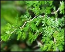
GoogLeNet was designed to tackle computer vision challenges involving Internet-quality image data, that is, images that have been captured in real contexts where the pose, lighting, occlusion, and clutter of images vary significantly. GoogLeNet was applied to the 2014 ImageNet challenge with noteworthy success, achieving only 6.7% error rate on the test dataset. ImageNet images are small, high-granularity images taken from many, varied classes. Multiple classes may appear very similar (such as varieties of tree) and the network architecture must be able to find increasingly challenging class distinctions to succeed. For a concrete example, consider the following ImageNet image:

Given the demands of this problem, the GoogLeNet architecture used to win ImageNet 14 departs from the LeNet model in several key ways. GoogLeNet's basic layer design is known as the Inception module and is made up of the following components:

The 1 x 1 convolutional layers used here are followed by Rectified Linear Units (ReLU). This approach is heavily used in speech and audio modeling contexts as ReLU can be used to effectively train deep models without pretraining and without facing some of the gradient vanishing problems that challenge other activation types. More information on ReLU is provided in the Further reading section of this chapter. The DepthConcat element provides a concatenation function, which consolidates the outputs of multiple units and substantially improves training time.

GoogLeNet chains layers of this type to create a full network. Indeed, the repetition of inception modules through GoogLeNet (nine times!) suggests that Network In Network (NIN) (deep architectures created from chained network modules) approaches are going to continue to be a serious contender in deep learning circles. The paper describing GoogLeNet and demonstrating how inception models were integrated into the network is provided in the Further reading section of this chapter.

Beyond the regularity of Inception module stacking, GoogLeNet has a few further surprises to throw at us. The first few layers are typically more straightforward with single-channel convolutional and max-pooling layers used at first. Additionally, at several points, GoogLeNet introduced a branch off the main structure using an average-pool layer, feeding into auxiliary softmax classifiers. The purpose of these classifiers was to improve the gradient signal that gets propagated back in lower layers of the network, enabling stronger performance at the early and middle network layers. Instead of one huge and potentially vague backpropagation process stemming from the final layer of the network, GoogLeNet instead has several intermediary update sources.

What's really important to take from this implementation is that GoogLeNet and other top convnet architectures are mainly successful because they are able to find effective configurations using the highly available components that we've discussed in this chapter. Now that we've had a chance to discuss the architecture and components of a convolutional net and the opportunity to discuss how these components are used to construct some highly advanced networks, it's time to apply the techniques to solve a problem of our own!