
The k-means algorithm is one of the most popular clustering algorithms. This algorithm is used to divide the input data into k subgroups using various attributes of the data. Grouping is achieved using an optimization technique where we try to minimize the sum of squares of distances between the datapoints and the corresponding centroid of the cluster. If you need a quick refresher, you can learn more about k-means at http://www.onmyphd.com/?p=k-means.clustering&ckattempt=1.
- The full code for this recipe is given in the
kmeans.pyfile already provided to you. Let's look at how it's built. Create a new Python file, and import the following packages:import numpy as np import matplotlib.pyplot as plt from sklearn import metrics from sklearn.cluster import KMeans import utilities
- Let's load the input data and define the number of clusters. We will use the
data_multivar.txtfile that's already provided to you:data = utilities.load_data('data_multivar.txt') num_clusters = 4 - We need to see what the input data looks like. Let's go ahead and add the following lines of the code to the Python file:
plt.figure()
plt.scatter(data[:,0], data[:,1], marker='o',
        facecolors='none', edgecolors='k', s=30)
x_min, x_max = min(data[:, 0]) - 1, max(data[:, 0]) + 1
y_min, y_max = min(data[:, 1]) - 1, max(data[:, 1]) + 1
plt.title('Input data')
plt.xlim(x_min, x_max)
plt.ylim(y_min, y_max)
plt.xticks(())
plt.yticks(())
If you run this code, you will get the following figure:

- We are now ready to train the model. Let's initialize the k-means object and train it:
kmeans = KMeans(init='k-means++', n_clusters=num_clusters, n_init=10)
kmeans.fit(data)
- Now that the data is trained, we need to visualize the boundaries. Let's go ahead and add the following lines of code to the Python file:
# Step size of the mesh
step_size = 0.01

# Plot the boundaries
x_min, x_max = min(data[:, 0]) - 1, max(data[:, 0]) + 1
y_min, y_max = min(data[:, 1]) - 1, max(data[:, 1]) + 1
x_values, y_values = np.meshgrid(np.arange(x_min, x_max, step_size), np.arange(y_min, y_max, step_size))

# Predict labels for all points in the mesh
predicted_labels = kmeans.predict(np.c_[x_values.ravel(), y_values.ravel()])
- We just evaluated the model across a grid of points. Let's plot these results to view the boundaries:
# Plot the results predicted_labels = predicted_labels.reshape(x_values.shape) plt.figure() plt.clf() plt.imshow(predicted_labels, interpolation='nearest', extent=(x_values.min(), x_values.max(), y_values.min(), y_values.max()), cmap=plt.cm.Paired, aspect='auto', origin='lower') plt.scatter(data[:,0], data[:,1], marker='o', facecolors='none', edgecolors='k', s=30) - Let's overlay the centroids on top of it:
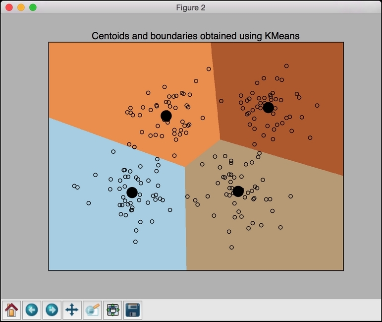
centroids = kmeans.cluster_centers_
plt.scatter(centroids[:,0], centroids[:,1], marker='o', s=200, linewidths=3,
        color='k', zorder=10, facecolors='black')
x_min, x_max = min(data[:, 0]) - 1, max(data[:, 0]) + 1
y_min, y_max = min(data[:, 1]) - 1, max(data[:, 1]) + 1
plt.title('Centoids and boundaries obtained using KMeans')
plt.xlim(x_min, x_max)
plt.ylim(y_min, y_max)
plt.xticks(())
plt.yticks(())
plt.show()
If you run this code, you should see the following figure:
..................Content has been hidden....................
You can't read the all page of ebook, please click here login for view all page.