The core algorithm for machine learning, gradient descent, is therefore revisited in order to adapt to online learning. When working on batch data, gradient descent can minimize the cost function of a linear regression analysis using much less computations than statistical algorithms. The complexity of gradient descent ranks in the order O(n*p), making learning regression coefficients feasible even in the occurrence of a large n (which stands for the number of observations) and large p (number of variables). It also works perfectly when highly correlated or even identical features are present in the training data.

Everything is based on a simple optimization method: the set of parameters is changed through multiple iterations in a way that it gradually converges to the optimal solution starting from a random one. Gradient descent is a theoretically well-understood optimization method with known convergence guarantees for certain problems such as regression ones. Nevertheless, let's start with the following image representing a complex mapping (typical of neural networks) between the values that the parameters can take (representing the hypothesis space) and result in terms of minimization of the cost function:

Using a figurative example, gradient descent resembles walking blindfolded around mountains. If you want to descend to the lowest valley without being able to see the path, you can just proceed by taking the direction that you feel is going downhill; try it for a while, then stop, feel the terrain again, and then proceed toward where you feel it is going downhill, and so on, again and again. If you keep on heading toward where the surface descends, you will finally arrive at a point when you cannot descend anymore because the terrain is flat. Hopefully, at that point, you should have reached your destination.

Using such a method, you need to perform the following actions:

In order to better depict what happens with gradient descent, let's take the example of a linear regression whose parameters are optimized by such a procedure.

We start from the cost function J given the vector of weights w:

The matrix-vector multiplication Xw between the training data matrix X and the vector of coefficients w represents the predictions from the linear model, whose deviance from the response y is squared, then summed, and finally divided by two times n, the number of instances.

Initially, the vector w could be instantiated using random numbers taken from the standardized normal distribution whose mean is zero and standard deviation is the unit. (Actually, initialization can be done in a lot of different ways, all working equally well to approximate linear regression whose cost function is bowl-shaped and has a unique minimum.) This allows our algorithm to start somewhere along the optimization path and could effectively speed up the convergence of the process. As we are optimizing a linear regression, initialization shouldn't cause much trouble to the algorithm (at worst, a wrong start will just slow it down). Instead, when we are using gradient descent in order to optimize different machine learning algorithms such as neural networks, we risk being stuck because of a wrong initialization. This will happen if, for instance, the initial w is just filled with zero values (the risk is getting stuck on a perfectly symmetric hilltop, where no directionality can immediately bring an optimization better than any other). This can happen with optimization processes that have multiple local minima, too.

Given the starting random coefficients vector w, we can immediately calculate the cost function J(w) and determine the initial direction for each single coefficient by subtracting from each a portion alpha (α, the learning rate) of the partial derivative of the cost function, as explicated by the following formula:

This can be better conveyed after solving the partial derivative, as follows:

Noticeably, the update is done on each singular coefficient (wj) given its feature vector xj, but based on all the predictions at once (hence the summation).

After iterating over all the coefficients in w, the coefficients' update will be completed and the optimization may restart again by calculating the partial derivative and updating the w vector.

An interesting characteristic of the process is that the update will be less and less as the w vector approaches the optimal configuration. Therefore, the process could stop when the change induced in w, with respect to the previous operation, is small. Anyway, it is true that we have decreasing updates when alpha, the learning rate, is set to the right size. In fact, if its value is too large, it may cause the optimization to detour and fail, causing—in some cases—a complete divergence of the process and the impossibility to converge finally to a solution. In fact, the optimization will tend to overshoot the target and actually get farther away from it.

At the other end, too small an alpha value will not only move the optimization process toward its target too slowly, but it may also be easily stuck somewhere in a local minima. This is especially true with regard to more complex algorithms, just like neural networks. As for linear regression and its classification counterpart, logistic regression, because the optimization curve is bowl-shaped, just like a concave curve, it features a single minimum and no local minima at all.

In the implementation that we illustrated, alpha is a fixed constant (a fixed learning rate gradient descent). As alpha plays such an important role in converging to an optimal solution, different strategies have been devised for it to start larger and shrink as the optimization goes on. We will discuss such different approaches when examining the Scikit-learn implementation.

The version of the gradient descent seen so far is known as full batch gradient descent and works by optimizing the error of the entire dataset, and thus needs it in-memory. The out-of-core versions are the stochastic gradient descent (SGD) and mini batch gradient descent.

Here, the formulation stays exactly the same, but for the update; the update is done for a single instance at a time, thus allowing us to leave the core data in its storage and take just a single observation in-memory:

The core idea is that, if the instances are picked randomly without particular biases, the optimization will move on average toward the target cost minimization. That explains why we discussed how to remove any ordering from a stream and making it as random as possible. For instance, in the bike-sharing example, if you have stochastic gradient descent learn the patterns of the early season first, then focus on the summer, then on the fall, and so on, depending on the season when the optimization is stopped, the model will be tuned to predict one season better than the others because most of the recent examples are from that season. In a stochastic gradient descent optimization, when data is independent and identically distributed (i.i.d.), convergence to the global minimum is guaranteed. Practically, i.i.d. means that your examples should have no sequential order or distribution but should be proposed to the algorithm as if picked randomly from your available ones.

A good number of online learning algorithms can be found in the Scikit-learn package. Not all machine learning algorithms have an online counterpart, but the list is interesting and steadily growing. As for supervised learning, we can divide available learners into classifiers and regressors and enumerate them.

As classifiers, we can mention the following:

As regressors, we have two options:

They all can learn incrementally, updating themselves instance by instance; though only SGDClassifier and SGDRegressor are based on the stochastic gradient descent optimization that we previously described, and they are the main topics of this chapter. The SGD learners are optimal for all large-scale problems as their complexity is bound to O(k*n*p), where k is the number of passes over the data, n is the number of instances, and p is the number of features (naturally non-zero features if we are working with sparse matrices): a perfectly linear time learner, taking more time exactly in proportion to the number of examples shown.

Other online algorithms will be used as a comparative benchmark. Moreover, all algorithms have the usage of the same API in common, based on the partial_fit method for online learning and mini-batch (when you stream larger chunks rather than a single instance). Sharing the same API makes all these learning techniques interchangeable in your learning frame.

Contrary to the fit method, which uses all the available data for its immediate optimization, partial_fit operates a partial optimization based on each of the single instances passed. Even if a dataset is passed to the partial_fit method, the algorithm won't process the entire batch but for its single elements, making the complexity of the learning operations indeed linear. Moreover, a learner, after partial_fit, can be perpetually updated by subsequent partial_fit calls, making it perfect for online learning from continuous streams of data.

When classifying, the only caveat is that at the first initialization, it is necessary to know how many classes we are going to learn and how they are labeled. This can be done using the classes parameter, pointing out a list of the numeric values labels. This requires to be explored beforehand, streaming through the data in order to record the labels of the problem and also taking notice of their distribution in case they are unbalanced—a class is numerically too large or too small with respect to the others (but the Scikit-learn implementation offers a way to automatically handle the problem). If the target variable is numeric, it is still useful to know its distribution, but this is not necessary to successfully run the learner.

In Scikit-learn, we have two implementations—one for classification problems (SGDClassifier) and one for regression ones (SGDRegressor). The classification implementation can handle multiclass problems using the one-vs-all (OVA) strategy. This strategy implies that, given k classes, k models are built, one for each class against all the instances of other classes, therefore creating k binary classifications. This will produce k sets of coefficients and k vectors of predictions and their probability. In the end, based on the emitted probability of each class compared against the other, the classification is assigned to the class with the highest probability. If we need to give actual probabilities for the multinomial distribution, we can simply normalize the results by dividing by their sum. (This is what is happening in a softmax layer in a neural network, which we will see in the following chapters.)

Both classification and regression SGD implementations in Scikit-learn feature different loss functions (the cost function, the core of the stochastic gradient descent optimization).

For classification, expressed by the loss parameter, we can rely on the following:

For regression, we have three loss functions:

We will present some examples using the classical statistical loss functions, which are logistic loss and OLS. Hinge loss and support vector machines (SVMs) will be discussed in the next chapter, a detailed introduction about their functioning being necessary.

As a reminder (so that you won't have to go and consult any other supplementary machine learning book), if we define the regression function as h and its predictions are given by h(X) because X is the matrix of features, then the following is the suitable formulation:

Consequently, the OLS cost function to be minimized is as follows:

In logistic regression, having a transformation of the binary outcome 0/1 into an odds ratio, πy being the probability of a positive outcome, the formula is as follows:

The logistic cost function, consequently, is defined as follows:

To define SGD parameters in Scikit-learn, both in classification and regression problems (so that they are valid for both SGDClassifier and SGDRegressor), we have to make clear how to deal with some important parameters necessary for a correct learning when you cannot evaluate all the data at once.

The first one is n_iter, which defines the number of iterations through the data. Initially set to 5, it has been empirically shown that it should be tuned in order for the learner, given the other default parameters, to see around 10^6 examples; therefore a good solution to set it would be n_iter = np.ceil(10**6 / n), where n is the number of instances. Noticeably, n_iter only works with in-memory datasets, so it acts only when you operate by the fit method but not with partial_fit. In reality, partial_fit will reiterate over the same data just if you restream it in your procedure and the right number of iterations of restreams is something to be tested along the learning procedure itself, being influenced by the type of data. In the next chapter, we will illustrate hyperparameter optimization and the right number of passes will be discussed.

shuffle is a parameter required if you want to shuffle your data. It refers to the mini-batch present in-memory and not to out-of-core data ordering. It also works with partial_fit but its effect in such a case is very limited. Always set it to True, but for data to be passed in chunks, shuffle your data out-of-core, as we described before.

warm_start is another parameter that works with the fit method because it remembers the previous fit coefficients (but not the learning rate if it has been dynamically modified). If you are using the partial_fit method, the algorithm will remember the previously learned coefficients and the state of the learning rate schedule.

The average parameter triggers a computational trick that, at a certain instance, starts averaging new coefficients with older ones allowing a faster convergence. It can be set to True or an integer value indicating from what instance it will start averaging.

Last, but not least, we have learning_rate and its related parameters, eta0 and power_t. The learning_rate parameter implies how each observed instance impacts on the optimization process. When presenting SGD from a theoretical point of view, we presented constant rate learning, which can be replicated setting learning_rate='constant'.

However, other options are present, letting the eta (called the learning rate in Scikit-learn and defined at time t) gradually decrease. In classification, the solution proposed is learning_rate='optimal', given by the following formulation:

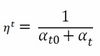
Here, t is the time steps, given by the number of instances multiplied by iterations, and t0 is a value heuristically chosen because of the studies by Léon Bottou, whose version of the Stochastic Gradient SVM has heavily influenced the SGD Scikit-learn implementation (http://leon.bottou.org/projects/sgd). The clear advantage of such a learning strategy is that learning decreases as more examples are seen, avoiding sudden perturbations of the optimization given by unusual values. Clearly, this strategy is also out-of-the-box, meaning that you don't have much to do with it.

In regression, the suggested learning fading is given by this formulation, corresponding to learning_rate= 'invscaling':

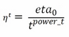
Here, eta0 and power_t are hyperparameters to be optimized by an optimization search (they are initially set to 0 and 0.5). Noticeably, using the invscaling learning rate, SGD will start with a lower learning rate, less than the optimal rate one, and it will decrease more slowly, being a bit more adaptable during learning.