
Between this and the previous chapter, we have come quite a long way covering the most important topics in deep learning. We now understand how to construct architectures by stacking multiple layers in a neural network and how to discern and utilize backpropagation methods. We also covered the concept of unsupervised pretraining with stacked and denoising autoencoders. The next and really exciting step in deep learning is the rapidly evolving field of Convolutional Neural Networks (CNN), a method of building multilayered, locally connected networks. CNNs, commonly referred to as ConvNets, are so rapidly evolving at the time of writing this book that we literally had to rewrite and update this chapter within a month's timeframe. In this chapter, we will cover the most fundamental and important concepts behind CNNs so that we will be able to run some basic examples without becoming overwhelmed by the sometimes enormous complexity. However, we won't be able to do justice fully to the enormous theoretical and computational background so this paragraph provides a practical starting point.
The best way to understand CNNs conceptually is to go back in history, start with a little bit of cognitive neuroscience, and look at Huber and Wiesel's research on the visual cortex of cats. Huber and Wiesel recorded neuro-activations of the visual cortex in cats while measuring neural activity by inserting microelectrodes in the visual cortex of the brain. (Poor cats!) They did this while the cats were watching primitive images of shapes projected on a screen. Interestingly, they found that certain neurons responded only to contours of specific orientation or shape. This led to the theory that the visual cortex is composed of local and orientation-specific neurons. This means that specific neurons respond only to images of specific orientation and shape (triangles, circles, or squares). Considering that cats and other mammals can perceive complex and evolving shapes into a coherent whole, we can assume that perception is an aggregate of all these locally and hierarchically organized neurons. By that time, the first multilayer perceptrons were already fully developed so it didn't take too long before this idea of locality and specific sensitivity in neurons was modeled in perceptron architectures. From a computational neuroscience perspective, this idea was developed into maps of local receptive regions in the brain with the addition of selectively connected layers. This was adopted by the already ongoing field of neural networks and artificial intelligence. The first reported scientist who applied this notion of local specific computationally to a multilayer perceptron was Fukushima with his so-called neocognitron (1982).
Yann LeCun developed the idea of the neocognitron into his version called LeNet. It added the gradient descent backpropagation algorithm. This LeNet architecture is still the foundation for many more evolved CNN architectures introduced recently. A basic CNN like LeNet learns to detect edges from raw pixels in the first layer, then use these edges to detect simple shapes in the second layer, and later in the process uses these shapes to detect higher-level features, such as objects in an environment in higher layers. The layer further down the neural sequence is then a final classifier that uses these higher-level features. We can see the feedforward pass in a CNN like this: we move from a matrix input to pixels, we detect edges from pixels, then shapes from edges, and detect increasingly distinctive and more abstract and complex features from shapes.
Note
Each convolution or layer in the network is receptive for a specific feature (such as shape, angle, or color).
Deeper layers will combine these features into a more complex aggregate. This way, it can process complete images without burdening the network with the full input space of the image at step.
Up until now, we have only worked with fully connected neural networks where each layer is connected to each neighboring layer. These networks have proven to be quite effective, but have the downside of dramatically increasing the number of parameters that we have to train. On a side note, we might imagine that when we train a small image (28 x 28) in size, we can get away with a fully connected network. However, training a fully connected network on larger images that span across the entire image would be tremendously computationally expansive.
Note
To summarize, we can state that CNNs have the following benefits over fully connected neural networks:
- They reduce the parameter space and thus prevent overtraining and computational load
- CNNs are invariant to object orientation (think of face recognition classifying faces with different locations)
- CNNs capable of learning and generalizing complex multidimensional features
- CNNs can be usefull in speech recogntion, image classification, and lately complex recommendation engines
CNNs utilize so-called receptive fields to connect the input to a feature map. The best way to understand CNNs is to dive deeper into the architecture, and of course get hands-on experience. So let's run through the types of layers that make up CNNs. The architecture of a CNN consists of three types of layers; namely, convolutional layer, pooling layer, and a fully-connected layer, where each layer accepts an input 3D volume (h, w, d) and transforms it into a 3D output through a differentiable function.
We can understand the concept of convolution by imagining a spotlight of a certain size sliding over the input (pixel-values and RGB color dimensions), conveniently after which we compute a dot product between the filtered values (also referred to as patches) and the true input. This does two important things: first, it compresses the input, and more importantly, second, the network learns filters that only activate when they see some specific type of feature spatial position in the input.
Look at the following image to see how this works:
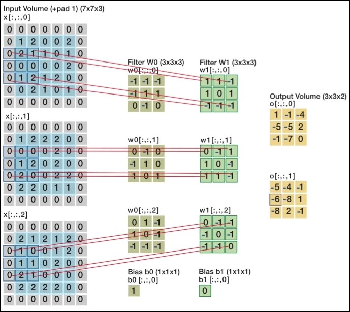
Two convolutional layers processing image input [7x7x3] input volume: an image of width 7, height 7, and with three color channels R,G,B
We can see from this image that we have two levels of filters (W0 and W1) and three dimensions (in the form of arrays) of inputs, all resulting in the dot product of the sliding spotlight/window over the input matrix. We refer to the size of this spotlight as stride, which means that the larger the stride, the smaller the output.
As you can see, when we apply a 3 x 3 filter, the full scope of the filter is processed at the center of the matrix, but once we move close to or past the edges, we start to lose out on the edges of the input. In this case, we apply what is called zero-padding. All elements that fall outside of the input dimensions are set to zero in this case. Zero-padding became more or less a default setting for most CNN applications recently.
The next type of layer that is often placed in between the filter layers is called a pooling layer or subsampling layer. What this does is it performs a downsampling operation along the spatial dimensions (width, height), which in turn helps with overfitting and reducing computational load. There are several ways to perform this downsampling, but recently Max Pooling turned out to be the most effective method.
Max-pooling is a simple method that compresses features by taking the maximum value of a patch of the neighboring feature. The following image will clarify this idea; each color box within the matrix represents a subsample of stride size 2:

A max-pooling layer with a stride of 2
The pooling layers are used mainly for the following reasons:
- Reduce the amount of parameters and thus computational load
- Regularization
Interestingly, the latest research findings suggest to leave out the pooling layer altogether, which will result in better accuracy (although at the expense of more strain on the CPU or GPU).
There is not much to explain about this type of layer. The final output where the classifications are computed (mostly with softmax) is a fully connected layer. However, in between convolutional layers, there (although rarely) are fully connected layers as well.
Before we apply a CNN ourselves, let's take what you have learned so far and inspect a CNN architecture to check our understanding. When we look at the ConvNet architecture in the following image, we can already get a sense of what a ConvNet will do to the input. The example is an effective convolutional neural network called AlexNet aimed at classifying 1.2 million images into 1,000 classes. It was used for the ImageNet contest in 2012. ImageNet is the most important image classification and localization competition in the world, which is held each year. AlexNet refers to Alex Krizhevsky (together with Vinod Nair and Geoffrey Hinton).

AlexNet architecture
When we look at the architecture, we can immediately see the input dimension 224 by 224 with three-dimensional depth. The stride size of four in the input, where max pooling layers are stacked, reduces the dimensionality of the input. In turn, this is followed by the convolutional layer. The two dense layers of size 4,096 are the fully connected layers leading to the final output that we mentioned before.
On a side note, we mentioned in a previous paragraph that TensorFlow's graph computation allows parallelization across GPUs. AlexNet did the same thing; look at the following image to see how they parallelized the architecture across GPUs:

The preceding image is taken from http://www.cs.toronto.edu/~fritz/absps/imagenet.pdf.
AlexNet let different models utilize GPUs by splitting up the architecture vertically to later be merged into the final classification output. That CNNs are more suitable for distributed processing is one of the biggest advantages of locally connected networks over fully connected ones. This model trained a set of 1.2 million images and took five days to complete on two NVIDIA GTX 580 3GB GPUs. Two multiple GPU units (a total of six GPUs) were used for this project.