
In this chapter, we'll continue building our skill with deep architectures by applying Stacked Denoising Autoencoders (SdA) to learn feature representations for high-dimensional input data.
We'll start, as before, by gaining a solid understanding of the theory and concepts that underpin autoencoders. We'll identify related techniques and call out the strengths of autoencoders as part of your data science toolkit. We'll discuss the use of Denoising Autoencoders (dA), a variation of the algorithm that introduces stochastic corruption to the input data, obliging the autoencoder to decorrupt the input and, in so doing, build a more effective feature representation.
We'll follow up on theory, as before, by walking through the code for a dA class, linking theory and implementation details to build a strong understanding of the technique.
At this point, we'll take a journey very similar to that taken in the preceding chapter—by stacking dA, we'll create a deep architecture that can be used to pretrain an MLP network, which offers substantial performance improvements in a range of unsupervised learning applications including speech data processing.
The autoencoder (also called the Diabolo network) is another crucial component of deep architectures. The autoencoder is related to the RBM, with autoencoder training resembling RBM training; however, autoencoders can be easier to train than RBMs with contrastive divergence and are thus preferred in contexts where RBMs train less effectively.
An autoencoder is a simple three-layer neural network whose output units are directly connected back to the input units. The objective of the autoencoder is to encode the i-dimensional input into an h-dimensional representation, where h < i, before reconstructing (decoding) the input at the output layer. The training process involves iteration over this process until the reconstruction error is minimized—at which point one should have arrived at the most efficient representation of input data (should, barring the possibility of arriving at local minima!).
In a preceding chapter, we discussed PCA as being a powerful dimensionality reduction technique. This description of autoencoders as finding the most efficient reduced-dimensional representation of input data will no doubt be familiar and you may be asking why we're exploring another technique that fulfils the same role.
The simple answer is that like the SOM, autoencoders can provide nonlinear reductions, which enables them to process high-dimensional input data more effectively than PCA. This revives a form of our earlier question—why discuss autoencoders if they deliver what an SOM does, without even providing the illuminating visual presentation?
Simply put, autoencoders are a more developed and sophisticated set of techniques; the use of denoising and stacking techniques enable reductions of high-dimensional, multimodal data that can be trained with relative ease to greater accuracy, at greater scale, than the techniques that we discussed in Chapter 1, Unsupervised Machine Learning.
Having discussed the capabilities of autoencoders at a high level, let's dig in a little further to understand the topology of autoencoders as well as what their training involves.
As described earlier in this chapter, an autoencoder has a relatively simple structure. It is a three-layer neural network, with input, hidden, and output layers. The input feeds forward into the hidden layer, then the output layer, as with most neural network architectures. One topological feature worth mentioning is that the hidden layer is typically of fewer nodes than the input or output layers. (However, as intimated previously, the required number of hidden nodes is really a function of the complexity of the input data; the goal of the hidden layer is to bottleneck the information content from the input and force the network to identify a representation that captures underlying statistical properties. Representing very complex input accurately might require a large quantity of hidden nodes.)
The key feature of an autoencoder is that the output is typically set to be the input; the performance measure for an autoencoder is its accuracy in reconstructing the input after encoding it within the hidden layer. Autoencoder topology tends to take the following form:

The encoding function that occurs between the input and hidden layers is a mapping of an input (x) to a new form (y). A simple example mapping function might be a nonlinear (in this case sigmoid, s) function of the input as follows:
However, more sophisticated encodings may exist or be developed to accommodate specific subject domains. In this case, of course, W represents the weight values assigned to x and b is an adjustable variable that can be tuned to enable the minimization of reconstruction error.
The autoencoder then decodes to deliver its output. This reconstruction is intended to take the same shape as x and will occur through a similar transformation as follows:
Here, b' and W' are typically also configurable to allow network optimization.
The network trains, as discussed, by minimizing the reconstruction error. One popular method to measure this error is a simple squared error measure, as shown in the following formula:

However, different and more appropriate error measures exist for cases where the input is in a less generic format (such as a set of bit probabilities).
While the intention is that autoencoders capture the main axes of variation in the input dataset, it is possible for an autoencoder to learn something far less useful—the identity function of the input.
While autoencoders can work well in some applications, they can be challenging to apply to problems where the input data contains a complex distribution that must be modeled in high dimensionality. The major challenge is that, with autoencoders that have n-dimensional input and an encoding of at least n, there is a real likelihood that the autoencoder will just learn the identity function of the input. In such cases, the encoding is a literal copy of the input. Such autoencoders are called overcomplete.
Note
One of the most important properties when training a machine learning technique is to understand how the dimensionality of hidden layers affects the quality of the resulting model. In cases where the input data is complex and the hidden layer has too few nodes to capture that complexity effectively, the result is obvious—the network fails to train as well as it might with more nodes.
To capture complex distributions in input data, then, you may wish to use a large number of hidden nodes. In cases where the hidden layer has at least as many nodes as the input, there is a strong possibility that the network will learn the identity of the input; in such cases, each element of the input is learned as a specific unique case. Naturally, a model that has been trained to do this will work very well over training data, but as it has learned a trivial pattern that cannot be generalized to unfamiliar data, it is liable to fail catastrophically when validated.
This is particularly relevant when modeling complex data, such as speech data. Such data is frequently complex in distribution, so the classification of speech signals requires multimodal encoding and a high-dimensional hidden layer. Of course, this brings an increased risk of the autoencoder (or any of a large number of models as this is not an autoencoder-specific problem) learning the identity function.
While (rather surprisingly) overcomplete autoencoders can and do learn error-minimizing representations under certain configurations (namely, ones in which the first hidden layer needs very small weights so as to force the hidden units into a linear orientation and subsequent weights have large values), such configurations are difficult to optimize for, and it has been desirable to find another way to prevent overcomplete autoencoders from learning the identity function.
There are several different ways that an overcomplete autoencoder can be prevented from learning the identity function while still capturing something useful within its representation. By far, the most popular approach is to introduce noise to the input data and force the autoencoder to train on the noisy data by learning distributions and statistical regularities rather than identity. This can be effectively achieved by multiple methods, including using sparseness constraints or dropout techniques (wherein input values are randomly set to zero).
The process that we'll be using to introduce noise to the input in this chapter is dropout. Via this method, up to half of the inputs are randomly set to zero. To achieve this, we create a stochastic corruption process that operates on our input data:
def get_corrupted_input(self, input, corruption_level):

   return self.theano_rng.binomial(size=input.shape, n=1, p=1 -
   corruption_level, dtype=theano.config.floatX) * input
In order to accurately model the input data, the autoencoder has to predict the corrupted values from the uncorrupted values, thus learning meaningful statistical properties (that is, distribution).
In addition to preventing an autoencoder from learning the identity values of data, adding a denoising process also tends to produce models that are substantially more robust to input variations or distortion. This proves to be particularly useful for input data that is inherently noisy, such as speech or image data. One commonly recognized advantage of deep learning techniques, mentioned in the preface to this book, is that deep learning algorithms minimize the need for feature engineering. Where many learning algorithms require lengthy and complicated preprocessing of input data (filtering of images or manipulation of audio signals) to reconstruct the denoised input and enable the model to train, a dA can work effectively with minimal preprocessing. This can dramatically decrease the time it takes to train a model over your input data to practical levels of accuracy.
Finally, it's worth observing that an autoencoder that learns the identity function of the input dataset is probably misconfigured in a fundamental way. As the main added value of the autoencoder is to find a lower-dimensional representation of the feature set, an autoencoder that has learned the identity function of the input data may simply have too many nodes. If in doubt, consider reducing the number of nodes in your hidden layer.
Now that we've discussed the topology of an autoencoder—the means by which one might be effectively trained and the role of denoising in improving autoencoder performance—let's review Theano code for a dA so as to carry the preceding theory into practice.
At this point, we're ready to step through the implementation of a dA. Once again, we're leveraging the Theano library to apply a dA class.
Unlike the RBM class that we explored in the previous chapter, the DenoisingAutoencoder is relatively simple and tying the functionality of the dA to the theory and math that we examined earlier in this chapter is relatively simple.
In Chapter 2, Deep Belief Networks, we applied an RBM class that had a number of elements that, while not necessary for the correct functioning of the RBM in itself, enabled shared parameters within multilayer, deep architectures. The dA class we'll be using possesses similar shared elements that will provide us with the means to build a multilayer autoencoder architecture later in the chapter.
We begin by initializing a dA class. We specify the number of visible units, n_visible, as well as the number of hidden units, n_hidden. We additionally specify variables for the configuration of the input (input) as well as the weights (W) and the hidden and visible bias values (bhid and bvis respectively). The four additional variables enable autoencoders to receive configuration parameters from other elements of a deep architecture:
class dA(object):
def __init__(
self,
numpy_rng,
theano_rng=None,
input=None,
n_visible=784,
n_hidden=500,
W=None,
bhid=None,
bvis=None
):
self.n_visible = n_visible
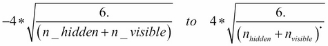
self.n_hidden = n_hiddenWe follow up by initialising the weight and bias variables. We set the weight vector, W to an initial value, initial_W, which we obtain using random, uniform sampling from the range:
We then set the visible and hidden bias variables to arrays of zeroes using numpy.zeros:
   if not theano_rng:
      theano_rng = RandomStreams(numpy_rng.randint(2 ** 30))

   if not W:
      initial_W = numpy.asarray(
         numpy_rng.uniform(
            low=-4 * numpy.sqrt(6. / (n_hidden + n_visible)),
            high=4 * numpy.sqrt(6. / (n_hidden + n_visible)),
            size=(n_visible, n_hidden)
         ),
         dtype=theano.config.floatX
      )
      W = theano.shared(value=initial_W, name='W', borrow=True)

   if not bvis:
      bvis = theano.shared(
         value=numpy.zeros(
            n_visible,
            dtype=theano.config.floatX
         ),
         borrow=True
      )

   if not bhid:
      bhid = theano.shared(
         value=numpy.zeros(
            n_hidden,
            dtype=theano.config.floatX
         ),
         name='b',
         borrow=True
      )
Earlier in the chapter, we described how the autoencoder translates between visible and hidden layers via mappings such as ![]() . To enable such translation, it is necessary to define
. To enable such translation, it is necessary to define W, b, W', and b' in relation to the previously described autoencoder parameters, bhid, bvis, and W. W' and b' are referred to as W_prime and b_prime in the following code:
self.W = W
self.b = bhid
self.b_prime = bvis
self.W_prime = self.W.T
self.theano_rng = theano_rng
if input is None:
   self.x = T.dmatrix(name='input')
else:
   self.x = input

self.params = [self.W, self.b, self.b_prime]
The preceding code sets b and b_prime to bhid and bvis respectively, while W_prime is set as the transpose of W; in other words, the weights are tied. Tied weights are sometimes, but not always, used in autoencoders for several reasons:
- Tying weights improves the quality of results in several contexts (albeit often in contexts where the optimal solution is PCA, which is the solution an autoencoder with tied weights will tend to reach)
- Tying weights improves the memory consumption of the autoencoder by reducing the number of parameters that need be stored
- Most importantly, tied weights provide a regularization effect; they require one less parameter to be optimized (thus one less thing that can go wrong!)
However, in other contexts, it's both common and appropriate to use untied weights. This is true, for instance, in cases where the input data is multimodal and the optimal decoder models a nonlinear set of statistical regularities. In such cases, a linear model, such as PCA, will not effectively model the nonlinear trends and you will tend to obtain better results using untied weights.
Having configured the parameters to our autoencoder, the next step is to define the functions that enable it to learn. Earlier in this chapter, we determined that autoencoders learn effectively by adding noise to input data, then attempting to learn an encoded representation of that input that can in turn be reconstructed into the input. What we need next, then, are functions that deliver this functionality. We begin by corrupting the input data:
def get_corrupted_input(self, input, corruption_level):

   return self.theano_rng.binomial(size=input.shape, n=1, p=1 –
   corruption_level, dtype=theano.config.floatX) * input
The degree of corruption is configurable using a corruption_level parameter; as we recognized earlier, the corruption of the input through dropout typically does not exceed 50% of cases, or 0.5. The function takes a random set of cases, where the number of cases is that proportion of the input whose size is equal to corruption_level. The function produces a corruption vector of 0's and 1's equal in length to the input, where a corruption_level sized proportion of the vector is 0. The corrupted input vector is then simply a multiple of the autoencoder's input vector and corruption vector:
def get_hidden_values(self, input):
   return T.nnet.sigmoid(T.dot(input, self.W) + self.b)
Next, we obtain the hidden values. This is done via code that performs the equation ![]() to obtain y (the hidden values). To get the autoencoder's output (z), we reconstruct the hidden layer via code that uses the previously defined
to obtain y (the hidden values). To get the autoencoder's output (z), we reconstruct the hidden layer via code that uses the previously defined b_prime and W_prime to perform ![]() :
:
defget_reconstructed_input(self, hidden):
   returnT.nnet.sigmoid(T.dot(hidden, self.W_prime) +
   self.b_prime)
The final missing piece is the calculation of cost updates. We reviewed one cost function previously, a simple squared error measure:  . Let's use this cost function to calculate our cost updates, based on the input (
x) and reconstruction (z):
def get_cost_updates(self, corruption_level, learning_rate):

   tilde_x = self.get_corrupted_input(self.x, corruption_level)
   y = self.get_hidden_values(tilde_x)
   z = self.get_reconstructed_input(y)
   E = (0.5 * (T.z – T.self.x)) ^ 2
   cost = T.mean(E)

   gparams = T.grad(cost, self.params)
   updates = [
      (param, param - learning_rate * gparam)
      for param, gparam in zip(self.params, gparams)
   ]

return (cost, updates)
At this point, we have a functional dA! It may be used to model nonlinear properties of input data and can work as an effective tool to learn valid and lower-dimensional representations of input data. However, the real power of autoencoders comes from the properties that they display when stacked together, as the building blocks of a deep architecture.