In H2O deep learning, the dataset that we will use to train is the famous MNIST dataset. It consists of pixel intensities of 28 x 28 images of handwritten digits. The training set has 70,000 training items with 784 features together with a label for each record containing the target label digits.

Now that we are more comfortable with managing data in H2O, let's perform a deep learning example.

In H2O, we don't have to transform or normalize the input data; it is standardized internally and automatically. Each feature is transformed into the N(0,1) space.

Let's import the famous handwritten digits image dataset MNIST from the Amazon server to the H2O cluster:

import h2o
h2o.init(start_h2o=True) 
train_url ="https://h2o-public-test-data.s3.amazonaws.com/bigdata/laptop/mnist/train.csv.gz"
test_url="https://h2o-public-test-data.s3.amazonaws.com/bigdata/laptop/mnist/test.csv.gz"


train=h2o.import_file(train_url)
test=h2o.import_file(test_url)

train.describe()
test.describe()


y='C785'
x=train.names[0:784]
train[y]=train[y].asfactor()
test[y]=test[y].asfactor()

from h2o.estimators.deeplearning import H2ODeepLearningEstimator

model_cv=H2ODeepLearningEstimator(distribution='multinomial'
                                 ,activation='RectifierWithDropout',hidden=[32,32,32],
                                        input_dropout_ratio=.2,
                                        sparse=True,
                                        l1=.0005,
                                            epochs=5)

The output of this print model will provide a lot of detailed information. The first table that you will see is the following one. This provides all the specifics about the architecture of the neural network. You can see that we have used a neural network with an input dimension of 717 with three hidden layers (consisting of 32 units each) with softmax activation applied to the output layer and ReLU between the hidden layers:

model_cv.train(x=x,y=y,training_frame=train,nfolds=3)
print model_cv

OUTPUT]

If you want a short overview of model performance, this is a very practical method.

In the following table, the most interesting metrics are the training classification error and validation classification error over each fold. You can easily compare these in case you want to validate your model:

    print model_cv.scoring_history()

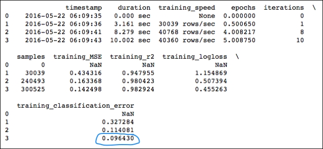
Our training classification error of .096430 and accuracy in the .907 range on the MNIST dataset is pretty good; it's almost as good as Yann LeCun's convolutional neural network submission.

H2O provides a convenient method to acquire validation metrics as well. We can do this by passing the validation dataframe to the cross-validation function:

model_cv.train(x=x,y=y,training_frame=train,validation_frame=test,nfolds=3)
print model_cv 

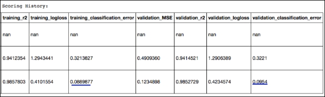
In this case, we can easily compare training_classification_error (.089) with our validation_classification_error (.0954).

Maybe we can improve our score; let's use a hyperparameter optimization model.

Considering that our previous model performed quite well, we will focus our tuning efforts on the architecture of our network. H2O's gridsearch function is quite similar to Scikit-learn's randomized search; namely, instead of searching the full parameter space, it iterates over a random list of parameters. First, we will set up a parameter list that we will pass to the gridsearch function. H2O will provide us with an output of each model and the corresponding score in the parameters' search:

hidden_opt = [[18,18],[32,32],[32,32,32],[100,100,100]]
# l1_opt = [s/1e6 for s in range(1,1001)]

# hyper_parameters = {"hidden":hidden_opt, "l1":l1_opt}
hyper_parameters = {"hidden":hidden_opt}

#important: here we specify the search parameters
#be careful with these, training time can explode (see max_models)
search_c = {"strategy":"RandomDiscrete",

"max_models":10, "max_runtime_secs":100,

"seed":222}


from h2o.grid.grid_search import H2OGridSearch

model_grid = H2OGridSearch(H2ODeepLearningEstimator, hyper_params=hyper_parameters)

#We have added a validation set to the gridsearch method in order to have a better #estimate of the model performance.
    

model_grid.train(x=x, y=y, distribution="multinomial", epochs=1000, training_frame=train, validation_frame=test,
    score_interval=2, stopping_rounds=3, stopping_tolerance=0.05,search_criteria=search_c)

print model_grid


# Grid Search Results for H2ODeepLearningEstimator:


OUTPUT]

deeplearning Grid Build Progress: [##################################################] 100%
    hidden  
0    [100, 100, 100]   
1       [32, 32, 32]   
2           [32, 32]   
3           [18, 18]   

    model_ids   logloss  
0  Grid_DeepLearning_py_1_model_python_1464790287811_3_model_3  0.148162  ←------
1  Grid_DeepLearning_py_1_model_python_1464790287811_3_model_2  0.173675  
2  Grid_DeepLearning_py_1_model_python_1464790287811_3_model_1  0.212246  
3  Grid_DeepLearning_py_1_model_python_1464790287811_3_model_0  0.227706  

We can see that our best architecture would be one with three layers with 100 units each. We can also clearly see that gridsearch increases training time substantially even on a powerful computing cluster like the one that H2O operates on. So, even on H2O, we should use gridsearch with caution and be conservative with the parameters that are parsed in the model.

Now let's shutdown the H2O instance before we proceed:

h2o.shutdown(prompt=False)