
We are now ready to build a deep neural network. A deep neural network consists of an input layer, many hidden layers, and an output layer. This looks like the following:

The preceding figure depicts a multilayer neural network with one input layer, one hidden layer, and one output layer. In a deep neural network, there are many hidden layers between the input and the output layers.
- Create a new Python file, and import the following packages:
import neurolab as nl
import numpy as np
import matplotlib.pyplot as plt
- Let's define parameters to generate some training data:
# Generate training data
min_value = -12
max_value = 12
num_datapoints = 90
- This training data will consist of a function that we define that will transform the values. We expect the neural network to learn this on its own, based on the input and output values that we provide:
x = np.linspace(min_value, max_value, num_datapoints)
y = 2 * np.square(x) + 7
y /= np.linalg.norm(y)
- Reshape the arrays:
data = x.reshape(num_datapoints, 1)
labels = y.reshape(num_datapoints, 1)
- Plot input data:
# Plot input data plt.figure() plt.scatter(data, labels) plt.xlabel('X-axis') plt.ylabel('Y-axis') plt.title('Input data') - Define a deep neural network with two hidden layers, where each hidden layer consists of 10 neurons:
# Define a multilayer neural network with 2 hidden layers;
# Each hidden layer consists of 10 neurons and the output layer
# consists of 1 neuron
multilayer_net = nl.net.newff([[min_value, max_value]], [10, 10, 1])
- Set the training algorithm to gradient descent (you can learn more about it at https://spin.atomicobject.com/2014/06/24/gradient-descent-linear-regression):
# Change the training algorithm to gradient descent
multilayer_net.trainf = nl.train.train_gd
- Train the network:
# Train the network
error = multilayer_net.train(data, labels, epochs=800, show=100, goal=0.01)
- Run the network on training data to see the performance:
# Predict the output for the training inputs
predicted_output = multilayer_net.sim(data)
- Plot the training error:
# Plot training error plt.figure() plt.plot(error) plt.xlabel('Number of epochs') plt.ylabel('Error') plt.title('Training error progress') - Let's create a set of new inputs and run the neural network on them to see how it performs:
# Plot predictions
x2 = np.linspace(min_value, max_value, num_datapoints * 2)
y2 = multilayer_net.sim(x2.reshape(x2.size,1)).reshape(x2.size)
y3 = predicted_output.reshape(num_datapoints)
- Plot the outputs:
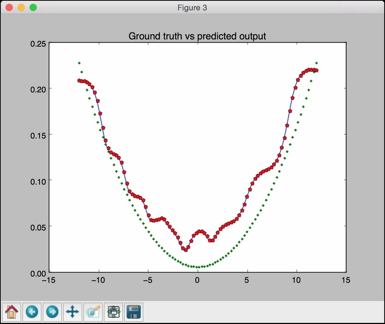
plt.figure() plt.plot(x2, y2, '-', x, y, '.', x, y3, 'p') plt.title('Ground truth vs predicted output') plt.show() - The full code is in the
deep_neural_network.pyfile that's already provided to you. If you run this code, you will see three figures. The first figure displays the input data:
The second figure displays the training error progress:

The third figure displays the output of the neural network:
You will see the following on your Terminal:
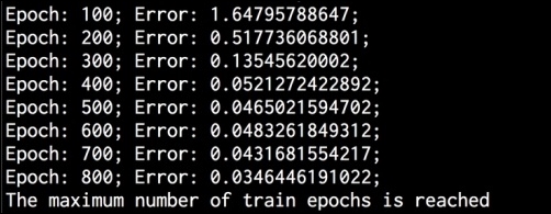
..................Content has been hidden....................
You can't read the all page of ebook, please click here login for view all page.