
Data streams pose the problem that you cannot evaluate as you would do when working on a complete in-memory dataset. For a correct and optimal approach to feed your SGD out-of-core algorithm, you first have to survey the data (by taking a chuck of the initial instances of the file, for example) and find out the type of data you have at hand.
We distinguish among the following types of data:
- Quantitative values
- Categorical values encoded with integer numbers
- Unstructured categorical values expressed in textual form
When data is quantitative, it could just be fed to the SGD learner but for the fact that the algorithm is quite sensitive to feature scaling; that is, you have to bring all the quantitative features into the same range of values or the learning process won't converge easily and correctly. Possible scaling strategies are converting all the values in the range [0,1], [-1,1] or standardizing the variable by centering its mean to zero and converting its variance to the unit. We don't have particular suggestions for the choice of the scaling strategy, but converting in the range [0,1] works particularly well if you are dealing with a sparse matrix and most of your values are zero.
As for in-memory learning, when transforming variables on the training set, you have to take notice of the values that you used (Basically, you need to get minimum, maximum, mean, and standard deviation of each feature.) and reuse them in the test set in order to achieve consistent results.
Given the fact that you are streaming data and it isn't possible to upload all the data in-memory, you have to calculate them by passing through all the data or at least a part of it (sampling is always a viable solution). The situation of working with an ephemeral stream (a stream you cannot replicate) poses even more challenging problems; in fact, you have to constantly keep trace of the values that you keep on receiving.
If sampling just requires you to calculate your statistics on a chunk of n instances (under the assumption that your stream has no particular order), calculating statistics on the fly requires you to record the right measures.
For minimum and maximum, you need to store a variable each for every quantitative feature. Starting from the very first value, which you will store as your initial minimum and maximum, for each new value that you will receive from the stream you will have to confront it with the previously recorded minimum and maximum values. If the new instance is out of the previous range of values, you just update your variable accordingly.
In addition, the average doesn't pose any particular problems because you just need to keep a sum of the values seen and a count of the instances. As for variance, you need to recall that the textbook formulation is as follows:
Noticeably, you need to know the mean μ, which you are also just learning incrementally from the stream. However, the formulation can be explicated as follows:
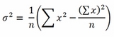
As you are just recording the number n of instances and a summation of x values, you just need to store another variable, which is the summation of values of x squared, and you will have all the ingredients for the recipe.
As an example, using the bike-sharing dataset, we can calculate the running mean, standard deviation, and range reporting the final result and plot how such stats changed as data was streamed from disk:
In: import os, csv
local_path = os.getcwd()
source = 'bikesharing\hour.csv'
SEP=','
running_mean = list()
running_std = list()
with open(local_path+''+source, 'rb') as R:
    iterator = csv.DictReader(R, delimiter=SEP)
    x = 0.0
    x_squared = 0.0
    for n, row in enumerate(iterator):
        temp = float(row['temp'])
        if n == 0:
            max_x, min_x = temp, temp
        else:
            max_x, min_x = max(temp, max_x),min(temp, min_x)
        x += temp
        x_squared += temp**2
        running_mean.append(x / (n+1))
        running_std.append(((x_squared - (x**2)/(n+1))/(n+1))**0.5)
        # DATA PROCESSING placeholder
        # MACHINE LEARNING placeholder
        pass
    print ('Total rows: %i' % (n+1))
    print ('Feature 'temp': mean=%0.3f, max=%0.3f, min=%0.3f, sd=%0.3f' % (running_mean[-1], max_x, min_x, running_std[-1]))

Out: Total rows: 17379
Feature 'temp': mean=0.497, max=1.000, min=0.020, sd=0.193
In a few moments, the data will be streamed from the source and key figures relative to the temp feature will be recorded as a running estimation of the mean and standard deviation is calculated and stored in two separated lists.
By plotting the values present in the lists, we can examine how much the estimates fluctuated with respect to the final figures and get an idea about how many instances are required before getting a stable mean and standard deviation estimate:
In: import matplotlib.pyplot as plt
%matplotlib inline
plt.plot(running_mean,'r-', label='mean')
plt.plot(running_std,'b-', label='standard deviation')
plt.ylim(0.0,0.6)
plt.xlabel('Number of training examples')
plt.ylabel('Value')
plt.legend(loc='lower right', numpoints= 1)
plt.show()
If you previously processed the original bike-sharing dataset, you will obtain a plot where clearly there is a trend in the data (due to temporal ordering, because the temperature naturally varies with seasons):

On the contrary, if we had used the shuffled version of the dataset as a source, the shuffled_hour.csv file, we could have obtained a couple of much more stable and quickly converging estimates. Consequently, we would have learned an approximate but more reliable estimate of the mean and standard deviation observing fewer instances from the stream:

The difference in the two charts reminds us of the importance of randomizing the order of the observations. Even learning simple descriptive statistics can be influenced heavily by trends in the data; consequently, we have to pay more attention when learning complex models by SGD.
In addition, the target variable also needs to be explored before starting. We need, in fact, to be sure about what values it assumes, if categorical, and figure out if it is unbalanced when in classes or has a skewed distribution when a number.
If we are learning a numeric response, we can adopt the same strategy shown previously for the features, whereas for classes, a Python dictionary keeping a count of classes (the keys) and their frequencies (the values) will suffice.
As an example, we will download a dataset for classification, the Forest Covertype data.
For a fast download and preparation of the data, we will use the gzip_from_UCI function as defined in the Datasets to try the real thing yourself section of the present chapter:
In: UCI_url = 'https://archive.ics.uci.edu/ml/machine-learning-databases/covtype/covtype.data.gz'
gzip_from_UCI(UCI_url)
In case of problems in running the code, or if you prefer to prepare the file by yourself, just go to the UCI website, download the dataset, and unpack it on the directory where Python is currently working:
https://archive.ics.uci.edu/ml/machine-learning-databases/covtype/
Once the data is available on disk, we can scan through the 581,012 instances, converting the last value of each row, representative of the class that we should estimate, to its corresponding forest cover type:
In: import os, csv
local_path = os.getcwd()
source = 'covtype.data'
SEP=','
forest_type = {1:"Spruce/Fir", 2:"Lodgepole Pine",
                3:"Ponderosa Pine", 4:"Cottonwood/Willow",
                5:"Aspen", 6:"Douglas-fir", 7:"Krummholz"}
forest_type_count = {value:0 for value in forest_type.values()}
forest_type_count['Other'] = 0
lodgepole_pine = 0
spruce = 0
proportions = list()
with open(local_path+''+source, 'rb') as R:
    iterator = csv.reader(R, delimiter=SEP)
    for n, row in enumerate(iterator):
        response = int(row[-1]) # The response is the last value
        try:
            forest_type_count[forest_type[response]] +=1
            if response == 1:
                spruce += 1
            elif response == 2:
                lodgepole_pine +=1
            if n % 10000 == 0:
                proportions.append([spruce/float(n+1),
                lodgepole_pine/float(n+1)])
        except:
            forest_type_count['Other'] += 1
    print ('Total rows: %i' % (n+1))
    print ('Frequency of classes:')
    for ftype, freq in sorted([(t,v) for t,v
        in forest_type_count.iteritems()], key =
        lambda x: x[1], reverse=True):
            print ("%-18s: %6i %04.1f%%" %
                    (ftype, freq, freq*100/float(n+1)))

Out: Total rows: 581012
Frequency of classes:
Lodgepole Pine    : 283301 48.8%
Spruce/Fir        : 211840 36.5%
Ponderosa Pine    :  35754 06.2%
Krummholz         :  20510 03.5%
Douglas-fir       :  17367 03.0%
Aspen             :   9493 01.6%
Cottonwood/Willow :   2747 00.5%
Other             :      0 00.0%
The output displays that two classes, Lodgepole Pine and Spruce/Fir, account for most observations. If examples are shuffled appropriately in the stream, the SGD will appropriately learn the correct a-priori distribution and consequently adjust its probability emission (a-posteriori probability).
If, contrary to our present case, your objective is not classification accuracy but increasing the receiver operating characteristic (ROC) area under the curve (AUC) or f1-score (error functions that can be used for evaluation; for an overview, you can directly consult the Scikit-learn documentation at http://scikit-learn.org/stable/modules/model_evaluation.html regarding a classification model trained on imbalanced data, and then the provided information can help you balance the weights using the class_weight parameter when defining SGDClassifier or sample_weight when partially fitting the model. Both change the impact of the observed instance by overweighting or underweighting it. In both ways, operating these two parameters will change the a-priori distribution. Weighting classes and instances will be discussed in the next chapter.
Before proceeding to training and working with classes, we can check whether the proportion of classes is always consistent in order to convey the correct a-priori probability to the SGD:
import matplotlib.pyplot as plt
import numpy as np
%matplotlib inline
proportions = np.array(proportions)
plt.plot(proportions[:,0],'r-', label='Spruce/Fir')
plt.plot(proportions[:,1],'b-', label='Lodgepole Pine')
plt.ylim(0.0,0.8)
plt.xlabel('Training examples (unit=10000)')
plt.ylabel('%')
plt.legend(loc='lower right', numpoints= 1)
plt.show()
In the previous figure, you can notice how the percentage of examples change as we progress streaming the data in the existing order. A shuffle is really necessary, in this case, if we want a stochastic online algorithm to learn correctly from data.
Actually, the proportions are changeable; this dataset has some kind of ordering, maybe a geographic one, that should be corrected by shuffling the data or we will risk overestimating or underestimating certain classes with respect to others.
If, among your features, there are categories (encoded in values or left in textual form), things can get a bit trickier. Normally, in batch learning, you would one-hot encode the categories and get as many new binary features as categories that you have. Unfortunately, in a stream, you do not know in advance how many categories you will deal with, and not even by sampling can you be sure of their number because rare categories may appear really late in the stream or require a too large sample to be discovered. You will have to first stream all the data and take a record of every category that appears. Anyway, streams can be ephemeral and sometimes the number of classes can be so large that they cannot be stored in-memory. The online advertising data is such an example because of its high volumes that are difficult to store away and because the stream cannot be passed over more than once. Moreover, advertising data is quite varied and features change constantly.
Working with texts makes the problem even more strikingly evident because you cannot anticipate what kind of word could be part of the text that you will be analyzing. In a bag-of-words model—where for each text the present words are counted and their frequency value pasted in an element in the feature vector specific to each word—you should be able to map each word to an index in advance. Even if you can manage this, you'll always have to handle the situation when an unknown word (therefore never mapped before) will pop up during testing or when the predictor is in production. Marginally, it should also be added that, being a spoken language, dictionaries made of hundreds of thousands or even millions of different terms are not unusual at all.
To recap, if you can handle knowing in advance the classes in your features, you can deal with them using the one-hot encoder from Scikit-learn (http://Scikit-learn.org/stable/modules/generated/sklearn.preprocessing.OneHotEncoder.html). We actually won't illustrate it here but basically the approach is not at all different from what you would apply when working with batch learning. What we want to illustrate to you is when you cannot really apply one-hot encoding.
There is a solution called the hashing trick because it is based on the hash function and can deal with both text and categorical variables in integer or string form. It can also work with categorical variables mixed with numeric values from quantitative features. The core problem with one-hot encoding is that it assigns a position to a value in the feature vector after having mapped its feature to that position. The hashing trick can univocally map a value to its position without any prior need to evaluate the feature because it leverages the core characteristic of a hashing function—to transform a value or string into an integer value deterministically.
Therefore, the only necessary preparation before applying it is creating a sparse vector large enough to represent the complexity of the data (potentially containing from 2**19 to 2**30 elements, depending on the available memory, bus architecture of your computer, and type of hash function that you are using). If you are working on some text, you'll also need a tokenizer, that is, a function that will split your text into single words and removes punctuation.
A simple toy example will make this clear. We will be using two specialized functions from the Scikit-learn package: HashingVectorizer, a transformer based on the hashing trick that works on textual data, and FeatureHasher, which is another transformer, specialized in converting a data row expressed as a Python dictionary to a sparse vector of features.
As the first example, we will turn a phrase into a vector:
In: from sklearn.feature_extraction.text import HashingVectorizer
h = HashingVectorizer(n_features=1000, binary=True, norm=None)
sparse_vector = h.transform(['A simple toy example will make clear how it works.'])
print(sparse_vector)

Out:
  (0, 61)       1.0
  (0, 271)      1.0
  (0, 287)      1.0
  (0, 452)      1.0
  (0, 462)      1.0
  (0, 539)      1.0
  (0, 605)      1.0
  (0, 726)      1.0
  (0, 918)      1.0
The resulting vector has unit values only at certain indexes, pointing out an association between a token in the phrase (a word) and a certain position in the vector. Unfortunately, the association cannot be reversed unless we map the hash value for each token in an external Python dictionary. Though possible, such a mapping would be indeed memory consuming because dictionaries can prove large, in the range of millions of items or even more, depending on the language and topics. Actually, we do not need to keep such tracking because hash functions guarantee to always produce the same index from the same token.
A real problem with the hashing trick is the eventuality of a collision, which happens when two different tokens are associated to the same index. This is a rare but possible occurrence when working with large dictionaries of words. On the other hand, in a model composed of millions of coefficients, there are very few that are influential. Consequently, if a collision happens, probably it will involve two unimportant tokens. When using the hashing trick, probability is on your side because with a large enough output vector (for instance, the number of elements is above 2^24), though collisions are always possible, it will be highly unlikely that they will involve important elements of the model.
The hashing trick can be applied to normal feature vectors, especially when there are categorical variables. Here is an example with FeatureHasher:
In: from sklearn.feature_extraction import FeatureHasher
h = FeatureHasher(n_features=1000, non_negative=True)
example_row = {'numeric feature':3, 'another numeric feature':2, 'Categorical feature = 3':1, 'f1*f2*f3':1*2*3}
print (example_row)

Out: {'another numeric feature': 2, 'f1*f2*f3': 6, 'numeric feature': 3, 'Categorical feature = 3': 1}
If your Python dictionary contains the feature names for numeric values and a composition of feature name and value for any categorical variable, the dictionary's values will be mapped using the hashed index of the keys creating a one-hot encoded feature vector, ready to be learned by an SGD algorithm:
In: print (h.transform([example_row]))
Out:
  (0, 16)       2.0
  (0, 373)      1.0
  (0, 884)      6.0
  (0, 945)      3.0
As we have drawn the example from our data storage, apart from turning categorical features into numeric ones, another transformation can be applied in order to have the learning algorithm increase its predictive power. Transformations can be applied to features by a function (by applying a square root, logarithm, or other transformation function) or by operations on groups of features.
In the next chapter, we will propose detailed examples regarding polynomial expansion and random kitchen-sink methods. In the present chapter, we will anticipate how to create quadratic features by nested iterations. Quadratic features are usually created when creating polynomial expansions and their aim is to intercept how predictive features interact between them; this can influence the response in the target variable in an unexpected way.
As an example to intuitively clarify why quadratic features can matter in modeling a target response, let's explain the case of the effect of two medicines on a patient. In fact, it could be that each medicine is effective, more or less, against the disease we are fighting against. Anyway, the two medicines are made up of different components that, when ingested together by the patient, tend to nullify each other's effect. In such a case, though both medicines are effective, but together they do not work at all because of their negative interaction.
In such a sense, interactions between features can be found among a large variety of features, not just in medicine, and it is critical to find out the most significant one in order for our model to work better in predicting its target. If we are not aware that certain features interact with respect to our problem, our only choice is to systematically test them all and have our model retain the ones that work better.
In the following simple example, a vector named v, an example we imagine has been just streamed in-memory in order to be learned is transformed into another vector vv where the original features of v are accompanied by the results of their multiplicative interactions (every feature is multiplied once by all the others). Given the larger number of features, the learning algorithm will be fed using the vv vector in place of the original v vector in order to achieve a better fit of the data:
In: import numpy as np
v = np.array([1, 2, 3, 4, 5, 6, 7, 8, 9, 10])
vv = np.hstack((v, [v[i]*v[j] for i in range(len(v)) for j in range(i+1, len(v))]))
print vv

Out:[ 1  2  3  4  5  6  7  8  9 10  2  3  4  5  6  7  8  9 10  6  8 10 12 14 16 18 20 12 15 18 21 24 27 30 20 24 28 32 36 40 30 35 40 45 50 42 48 54 60 56 63 70 72 80 90]
Similar transformations, or even more complex ones, can be generated on the fly as the examples stream to the learning algorithm, exploiting the fact that the data batch is small (sometimes reduced to single examples) and expanding the number of features of so a few examples can feasibly be achieved in-memory. In the following chapter, we will explore more examples of such transformations and their successful integration into the learning pipeline.
We have withheld showing full examples of training after introducing SGD because we need to introduce how to test and validate in a stream. Using batch learning, testing, and cross-validating is a matter of randomizing the order of the observations, slicing the dataset into folds and taking a precise fold as a test set, or systematically taking all the folds in turn to test your algorithm's learning capabilities.
Streams cannot be kept in-memory, so on the basis that the following instances are already randomized, the best solution is to take validation instances after the stream has unfolded for a while or systematically use a precise, replicable pattern in the data stream.
An out-of-sample approach on part of a stream is actually comparable to a test sample and can be successfully accomplished only knowing in advance the length of the stream. For continuous streams, it is still possible but implies stopping the learning definitely once the test instances start. This method is called a holdout after n strategy.
A cross-validation type of approach is possible using a systematic and replicable sampling of validation instances. After having defined a starting buffer, an instance is picked for validation every n times. Such an instance is not used for the training but for testing purposes. This method is called a periodic holdout strategy every n times.
As validation is done on a single instance base, a global performance measure is calculated, averaging all the error measures collected so far within the same pass over the data or in a window-like fashion, using the most recent set of k measures, where k is a number of tests that you think is validly representative.
As a matter of fact, during the first pass, all instances are actually unseen to the learning algorithm. It is therefore useful to test the algorithm as it receives cases to learn, verifying its response on an observation before learning it. This approach is called progressive validation.
As a conclusion of the present chapter, we will implement two examples: one for classification based on the Forest Covertype data and one for regression based on the bike-sharing dataset. We will see how to put into practice the previous insights on response and feature distributions and how to use the best validation strategy for each problem.
Starting with the classification problem, there are two noticeable aspects to consider. Being a multiclass problem, first of all we noticed that there is some kind of ordering in the database and distribution of classes along the stream of instances. As an initial step, we will shuffle the data using the ram_shuffle function defined during the chapter in the Paying attention to the ordering of instances section:
In: import os
local_path = os.getcwd()
source = 'covtype.data'
ram_shuffle(filename_in=local_path+''+source,
            filename_out=local_path+'\shuffled_covtype.data',
            header=False)
As we are zipping the rows in-memory and shuffling them without much disk usage, we can quickly obtain a new working file. The following code will train SGDClassifier with log loss (equivalent to a logistic regression) so that it leverages our previous knowledge of the classes present in the dataset. The forest_type list contains all the codes of the classes and it is passed every time (though just one, the first, would suffice) to the partial_fit method of the SGD learner.
For validation purposes, we define a cold start at 200.000 observed cases. At every ten instances, one will be left out of training and used for validation. This schema allows reproducibility even if we are going to pass over the data multiple times; at every pass, the same instances will be left out as an out-of-sample test, allowing the creation of a validation curve to test the effect of multiple passes over the same data.
The holdout schema is accompanied by a progressive validation, too. So each case after the cold start is evaluated before being fed to the training. Although progressive validation provides an interesting feedback, such an approach will work only for the first pass; in fact after the initial pass, all the observations (but the ones in the holdout schema) will become in-sample instances. In our example, we are going to make only one pass.
As a reminder, the dataset has 581.012 instances and it may prove a bit long to stream and model with SGD (it is quite a large-scale problem for a single computer). Though we placed a limiter to observe just 250.000 instances, still allow your computer to run for about 15-20 minutes before expecting results:
In: import csv, time
import numpy as np
from sklearn.linear_model import SGDClassifier
source = 'shuffled_covtype.data'
SEP=','
forest_type = [t+1 for t in range(7)]
SGD = SGDClassifier(loss='log', penalty=None, random_state=1, average=True)
accuracy = 0
holdout_count = 0
prog_accuracy = 0
prog_count = 0
cold_start = 200000
k_holdout = 10
with open(local_path+''+source, 'rb') as R:
    iterator = csv.reader(R, delimiter=SEP)
    for n, row in enumerate(iterator):
        if n > 250000: # Reducing the running time of the experiment
            break
        # DATA PROCESSING
        response = np.array([int(row[-1])]) # The response is the last value
        features = np.array(map(float,row[:-1])).reshape(1,-1)
        # MACHINE LEARNING
        if (n+1) >= cold_start and (n+1-cold_start) % k_holdout==0:
            if int(SGD.predict(features))==response[0]:
                accuracy += 1
            holdout_count += 1
            if (n+1-cold_start) % 25000 == 0 and (n+1) > cold_start:
                    print '%s holdout accuracy: %0.3f' % (time.strftime('%X'), accuracy / float(holdout_count))
        else:
            # PROGRESSIVE VALIDATION
            if (n+1) >= cold_start:
                if int(SGD.predict(features))==response[0]:
                    prog_accuracy += 1
                prog_count += 1
                if n % 25000 == 0 and n > cold_start:
                    print '%s progressive accuracy: %0.3f' % (time.strftime('%X'), prog_accuracy / float(prog_count))
            # LEARNING PHASE
            SGD.partial_fit(features, response, classes=forest_type)
print '%s FINAL holdout accuracy: %0.3f' % (time.strftime('%X'), accuracy / ((n+1-cold_start) / float(k_holdout)))
print '%s FINAL progressive accuracy: %0.3f' % (time.strftime('%X'), prog_accuracy / float(prog_count))

Out:
18:45:10 holdout accuracy: 0.627
18:45:10 progressive accuracy: 0.613
18:45:59 holdout accuracy: 0.621
18:45:59 progressive accuracy: 0.617
18:45:59 FINAL holdout accuracy: 0.621
18:45:59 FINAL progressive accuracy: 0.617
As the second example, we will try to predict the number of shared bicycles in Washington based on a series of weather and time information. Given the historical order of the dataset, we do not shuffle it and treat the problem as a time series one. Our validation strategy is to test the results after having seen a certain number of examples in order to replicate the uncertainities to forecast from that moment of time onward.
It is also interesting to notice that some of the features are categorical, so we applied the FeatureHasher class from Scikit-learn in order to represent having the categories recorded in a dictionary as a joint string made up of the variable name and category code. The value assigned in the dictionary for each of these keys is one in order to resemble a binary variable in the sparse vector that the hashing trick will be creating:
In: import csv, time, os
import numpy as np
from sklearn.linear_model import SGDRegressor
from sklearn.feature_extraction import FeatureHasher
source = '\bikesharing\hour.csv'
local_path = os.getcwd()
SEP=','
def apply_log(x): return np.log(float(x)+1)
def apply_exp(x): return np.exp(float(x))-1
SGD = SGDRegressor(loss='squared_loss', penalty=None, random_state=1, average=True)
h = FeatureHasher(non_negative=True)
val_rmse = 0
val_rmsle = 0
predictions_start = 16000
with open(local_path+''+source, 'rb') as R:
    iterator = csv.DictReader(R, delimiter=SEP)
    for n, row in enumerate(iterator):
        # DATA PROCESSING
        target = np.array([apply_log(row['cnt'])])
        features = {k+'_'+v:1 for k,v in row.iteritems()
        if k in ['holiday','hr','mnth','season',
           'weathersit','weekday','workingday','yr']}
        numeric_features = {k:float(v) for k,v in
           row.iteritems() if k in ['hum', 'temp', '
           atemp', 'windspeed']}
        features.update(numeric_features)
        hashed_features = h.transform([features])
        # MACHINE LEARNING
        if (n+1) >= predictions_start:
            # HOLDOUT AFTER N PHASE
            predicted = SGD.predict(hashed_features)
            val_rmse += (apply_exp(predicted)
               - apply_exp(target))**2
            val_rmsle += (predicted - target)**2
            if (n-predictions_start+1) % 250 == 0
               and (n+1) > predictions_start:
                  print '%s holdout RMSE: %0.3f'
                     % (time.strftime('%X'), (val_rmse
                     / float(n-predictions_start+1))**0.5),
                print 'holdout RMSLE: %0.3f' % ((val_rmsle
/ float(n-predictions_start+1))**0.5)
        else:
            # LEARNING PHASE
            SGD.partial_fit(hashed_features, target)

print '%s FINAL holdout RMSE: %0.3f' %
(time.strftime('%X'), (val_rmse
    / float(n-predictions_start+1))**0.5)
print '%s FINAL holdout RMSLE: %0.3f' %
(time.strftime('%X'), (val_rmsle
    / float(n-predictions_start+1))**0.5)

Out:
18:02:54 holdout RMSE: 281.065 holdout RMSLE: 1.899
18:02:54 holdout RMSE: 254.958 holdout RMSLE: 1.800
18:02:54 holdout RMSE: 255.456 holdout RMSLE: 1.798
18:52:54 holdout RMSE: 254.563 holdout RMSLE: 1.818
18:52:54 holdout RMSE: 239.740 holdout RMSLE: 1.737
18:52:54 FINAL holdout RMSE: 229.274
18:52:54 FINAL holdout RMSLE: 1.678