Before starting, it is important to know that there are two main branches of Python: versions 2 and 3. As many core functionalities have changed, scripts built for one version are sometimes incompatible with the other one (they won't work without raising errors and warnings). Although the third version is the newest, the older one is still the most used version in the scientific area and the default version for many operative systems (mainly for compatibility in upgrades). When version 3 was released (in 2008), most scientific packages weren't ready so the scientific community stuck with the previous version. Fortunately, since then, almost all packages have been updated leaving just a few (see http://py3readiness.org for a compatibility overview) as orphans of Python 3 compatibility.

In spite of the recent growth in popularity of Python 3 (which, we shouldn't forget, is the future of Python), Python 2 is still widely used among data scientists and data analysts. Moreover, for a long time Python 2 has been the default Python installation (for instance, on Ubuntu), so it is the most likely version that most of the readers should have ready at hand. For all these reasons, we will adopt Python 2 for this book. It is not merely love for the old technologies, it is just a practical choice in order to make Large Scale Machine Learning with Python accessible to the largest audience:

More often than not, you will find yourself in a situation where you have to upgrade a package because the new version is either required by a dependency or has additional features that you would like to use. To do so, first check the version of the library that you have installed by glancing at the __version__ attribute, as shown in the following example using the NumPy package:

>>> import numpy
>>> numpy.__version__ # 2 underscores before and after
'1.9.0'

Now, if you want to update it to a newer release, say precisely the 1.9.2 version, you can run the following command from the command line:

$ pip install -U numpy==1.9.2

Alternatively (but we do not recommend it unless it proves necessary), you can also use the following command:

$ easy_install --upgrade numpy==1.9.2

Finally, if you're just interested in upgrading it to the latest available version, simply run the following command:

$ pip install -U numpy

You can also run the easy_install alternative:

$ easy_install --upgrade numpy

As you've read so far, creating a working environment is a time-consuming operation for a data scientist. You first need to install Python and then, one by one, you can install all the libraries that you will need. (Sometimes, the installation procedures may not go as smoothly as you'd hoped for earlier.)

If you want to save time and effort and want to ensure that you have a fully working Python environment that is ready to use, you can just download, install, and use the scientific Python distribution. Apart from Python, they also include a variety of preinstalled packages, and sometimes they even have additional tools and an IDE setup for your usage. A few of them are very well-known among data scientists, and in the sections that follow, you will find some of the key features for two of these packages that we found most useful and practical.

To immediately focus on the contents of the book, we suggest that you first promptly download and install a scientific distribution, such as Anaconda (which is the most complete one around, in our opinion), and decide to fully uninstall the distribution and set up Python alone after practicing the examples in the book, which can be accompanied by just the packages you need for your projects.

Again, if possible, download and install the version containing Python 3.

The first package that we would recommend you to try is Anaconda (https://www.continuum.io/downloads), which is a Python distribution offered by Continuum Analytics that includes nearly 200 packages, including NumPy, SciPy, pandas, IPython, matplotlib, Scikit-learn, and StatsModels. It's a cross-platform distribution that can be installed on machines with other existing Python distributions and versions, and its base version is free. Additional add-ons that contain advanced features are charged separately. Anaconda introduces conda, a binary package manager, as a command-line tool to manage your package installations. As stated on its website, Anaconda's goal is to provide enterprise-ready Python distribution for large-scale processing, predictive analytics and scientific computing. As for Python version 2.7, we recommend the Anaconda distribution 4.0.0. (In order to have a look at the packages installed with Anaconda, you can have a look at the list at https://docs.continuum.io/anaconda/pkg-docs.)

As a second suggestion, if you are working on Windows and you desire a portable distribution, WinPython (http://winpython.sourceforge.net/) could be a quite interesting alternative (sorry, no Linux or MacOS versions). WinPython is also a free, open source Python distribution maintained by the community. It is also designed with scientists in mind, and it includes many essential packages such as NumPy, SciPy, matplotlib, and IPython (basically the same as Anaconda's). It also includes Spyder as an IDE, which can be helpful if you have experience using the MATLAB language and interface. Its crucial advantage is that it is portable (you can put it in any directory or even in a USB flash drive), so you can have different versions present on your computer, move a version from a Windows computer to another, and you can easily replace an older version with a newer one just by replacing its directory. When you run WinPython or its shell, it will automatically set all the environment variables necessary to run Python as if it were regularly installed and registered on your system.

IPython was initiated in 2001 as a free project by Fernando Perez, addressing a lack in the Python stack for scientific investigations using a user-programming interface that could incorporate the scientific approach (mainly experimenting and interactively discovering) in the process of software development.

A scientific approach implies the fast experimentation of different hypotheses in a reproducible fashion (as does the data exploration and analysis task in data science), and when using IPython, you will be able to implement an explorative, iterative, and trial-and-error research strategy more naturally during your code writing.

Recently, a large part of the IPython project has moved to a new one called Jupyter. This new project extends the potential usability of the original IPython interface to a wide range of programming languages. (For a complete list, visit https://github.com/ipython/ipython/wiki/IPython-kernels-for-other-languages.)

Thanks to the powerful idea of kernels, programs that run the user's code are communicated by the frontend interface and provide feedback on the results of the executed code to the interface itself; you can use the same interface and interactive programming style, no matter what language you are developing in.

Jupyter (IPython is the zero kernel, the original starting one) can be simply described as a tool for interactive tasks operable by a console or web-based notebook, which offers special commands that help developers better understand and build the code that is being currently written.

Contrary to an IDE, which is built around the idea of writing a script, running it afterward and evaluating its results, Jupyter lets you write your code in chunks named cells, run each of them sequentially, and evaluate the results of each one separately, examining both textual and graphic outputs. Besides graphical integration, it provides you with further help, thanks to customizable commands, a rich history (in the JSON format), and computational parallelism for an enhanced performance when dealing with heavy numeric computations.

Such an approach is also particularly fruitful for the tasks involving developing code based on data as it automatically accomplishes the often neglected duty of documenting and illustrating how data analysis has been done, its premises and assumptions, and its intermediate and final results. If a part of your job is to also present your work and persuade internal or external stakeholders to the project, Jupyter can really do the magic of storytelling for you with few additional efforts. There are many examples on https://github.com/ipython/ipython/wiki/A-gallery-of-interesting-IPython-Notebooks, some of which you may find inspiring for your work as we did.

Actually, we have to confess that keeping a clean, up-to-date Jupyter Notebook has saved us uncountable times when meetings with managers/stakeholders have suddenly popped up, requiring us to hastily present the state of our work.

In short, Jupyter offers you the following features:

Jupyter is our favored choice throughout this book, and it is used to clearly and effectively illustrate storytelling operations with scripts and data and their consequent results.

Though we strongly recommend using Jupyter, if you are using an REPL or IDE, you can use the same instructions and expect identical results (except for print formats and extensions of the returned results).

If you do not have Jupyter installed on your system, you can promptly set it up using the following command:

$ pip install jupyter

If you already have Jupyter installed, it should be upgraded to at least version 4.1.

After installation, you can immediately start using Jupyter, calling it from the command line:

$ jupyter notebook

Once the Jupyter instance has opened in the browser, click on the New button, and in the Notebooks section, choose Python 2 (other kernels may be present in the section, depending on what you installed):

At this point, your new empty notebook will look like the following screenshot and you can start entering the commands in the cells:

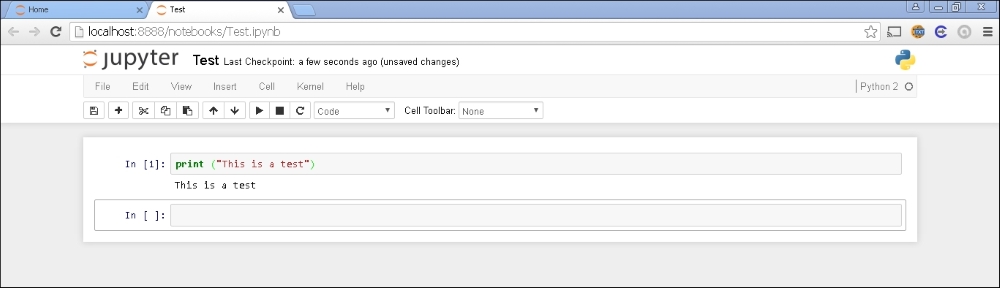
For instance, you may start typing the following in the cell:

In: print ("This is a test")

After writing in cells, you just press the play button (below the Cell tab) to run it and obtain an output. Then, another cell will appear for your input. As you are writing in a cell, if you press the plus button on the above menu bar, you will get a new cell, and you can move from a cell to another using the arrows on the menu.

Most of the other functions are quite intuitive and we invite you to try them. In order to know better how Jupyter works, you may use a quick-start guide such as http://jupyter-notebook-beginner-guide.readthedocs.io/en/latest/ or you can get a book specialized in Jupyter functionalities.

For our illustrative purposes, just consider that every Jupyter block of instructions has a numbered input statement and an output one, so you will find the code presented in this book structured in to two blocks—at least when the output is not trivial at all—otherwise, just expect only the input part:

In:  <the code you have to enter>
Out: <the output you should get>

As a rule, you just have to type the code after In: in your cells and run it. You can then compare your output with the output that we provide using Out: followed by the output that we actually obtained on our computers when we tested the code.