
Let's start our neural network adventure with a perceptron. A perceptron is a single neuron that performs all the computation. It is a very simple model, but it forms the basis of building up complex neural networks. Here is what it looks like:

The neuron combines the inputs using different weights, and it then adds a bias value to compute the output. It's a simple linear equation relating input values with the output of the perceptron.
- Create a new Python file, and import the following packages:
import numpy as np
import neurolab as nl
import matplotlib.pyplot as plt
- Define some input data and their corresponding labels:
# Define input data
data = np.array([[0.3, 0.2], [0.1, 0.4], [0.4, 0.6], [0.9, 0.5]])
labels = np.array([[0], [0], [0], [1]])
- Let's plot this data to see where the datapoints are located:
# Plot input data plt.figure() plt.scatter(data[:,0], data[:,1]) plt.xlabel('X-axis') plt.ylabel('Y-axis') plt.title('Input data') - Let's define a
perceptronwith two inputs. This function also needs us to specify the minimum and maximum values in the input data:# Define a perceptron with 2 inputs; # Each element of the list in the first argument # specifies the min and max values of the inputs perceptron = nl.net.newp([[0, 1],[0, 1]], 1)
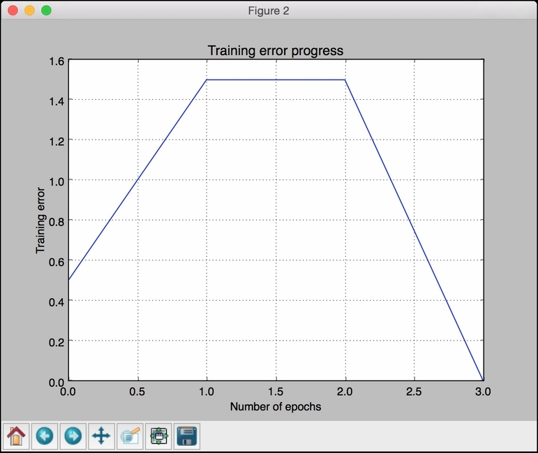
- Let's train the perceptron. The number of epochs specifies the number of complete passes through our training dataset. The
showparameter specifies how frequently we want to display the progress. Thelrparameter specifies the learning rate of the perceptron. It is the step size for the algorithm to search through the parameter space. If this is large, then the algorithm may move faster, but it might miss the optimum value. If this is small, then the algorithm will hit the optimum value, but it will be slow. So it's a trade-off; hence, we choose a value of0.01:# Train the perceptron error = perceptron.train(data, labels, epochs=50, show=15, lr=0.01)
- Let's plot the results, as follows:
# plot results plt.figure() plt.plot(error) plt.xlabel('Number of epochs') plt.ylabel('Training error') plt.grid() plt.title('Training error progress') plt.show() - The full code is given in the
perceptron.pyfile that's already provided to you. If you run this code, you will see two figures. The first figure displays the input data: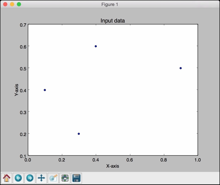
The second figure displays the training error progress:
..................Content has been hidden....................
You can't read the all page of ebook, please click here login for view all page.