
In this chapter, we will focus on scalable methods for classification and regression trees. The following topics will be covered:
- Tips and tricks for fast random forest applications in Scikit-learn
- Additive random forest models and subsampling
- GBM gradient boosting
- XGBoost together with streaming methods
- Very fast GBM and random forest in H2O
The aim of a decision tree is to learn a series of decision rules to infer the target labels based on the training data. Using a recursive algorithm, the process starts at the tree root and splits the data on the feature that results in the lowest impurity. Currently, the most widely applicable scalable tree-based applications are based on CART. Introduced by Breiman, Friedman Stone, and Ohlson in 1984, CART is an abbreviation of Classification and Regression Trees. CART is different from other decision tree models (such as ID3, C4.5/C5.0, CHAID, and MARS) in two ways. First, CART is applicable to both classification and regression problems. Second, it builds binary trees (at each split, resulting in a binary split). This enables CART trees to operate recursively on given features and optimize in a greedy fashion on an error metric in the form of impurity. These binary trees together with scalable solutions are the focus of this chapter.
Let's look closely at how these trees are constructed. We can see a decision tree as a graph with nodes, passing information down from top to bottom. Each decision within the tree is made by binary splits for either classes (Boolean) or continuous variables (a threshold value) resulting in a final prediction.
Trees are constructed and learned by the following procedure:
- Recursively finding the variable that best splits the target label from root to terminal node. This is measured by the impurity of each feature that we minimize based on the target outcome. In this chapter, the relevant impurity measures are Gini impurity and cross entropy.
Gini impurity
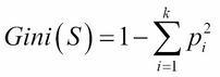
Gini impurity is a metric that measures the divergence between the probability pi of the target classes (k) so that an equal spread of probability values over the target classes result in a high Gini impurity.
Cross entropy
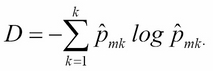
With cross entropy, we look at the log probability of misclassification. Both metrics are proven to yield quite similar results. However, Gini impurity is computationally more efficient because it does not require calculating the logs.
We do this until a stopping criterion is met. This criteria can roughly mean two things: one, adding new variables no longer improves the target outcome, and second, a maximum tree depth or tree complexity threshold is reached. Note that very deep and complex trees with many nodes can easily lead to overfitting. In order to prevent this, we generally prune the tree by limiting the tree depth.
To get an intuition for how this process works, let's build a decision tree with Scikit-learn and visualize it with graphviz. First, create a toy dataset to see if we can predict who is a smoker and who is not based on IQ (numeric), age (numeric), annual income (numeric), business owner (Boolean), and university degree (Boolean). You need to download the software from http://www.graphviz.org in order to load a visualization of the tree.dot file that we are going to create with Scikit-learn:
import numpy as np
from sklearn import tree
iq=[90,110,100,140,110,100]
age=[42,20,50,40,70,50]
anincome=[40,20,46,28,100,20]
businessowner=[0,1,0,1,0,0]
univdegree=[0,1,0,1,0,0]
smoking=[1,0,0,1,1,0]
ids=np.column_stack((iq, age, anincome,businessowner,univdegree))
names=['iq','age','income','univdegree']
dt = tree.DecisionTreeClassifier(random_state=99)
dt.fit(ids,smoking)
dt.predict(ids)
tree.export_graphviz(dt,out_file='tree2.dot',feature_names=names,label=all,max_depth=5,class_names=True)
You can now find the tree.dot file in your working directory. Once you find this file, you can open it with the graphviz software:
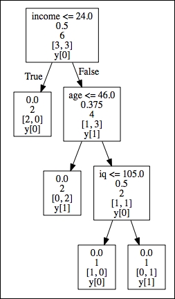
- Root node (Income): This is the starting node that represents the feature with the highest information gain and lowest impurity (Gini=.5)
- Internal nodes (Age and IQ):This is each node between the root node and terminal. Parent nodes pass down decision rules to the receiving end—child nodes (left and right)
- Terminal nodes (leaf nodes): The target labels partitioned by the tree structure
Tree-depth is the number of edges from the root node to the terminal nodes. In this case, we have a tree depth of 3.
We can now see all the binary splits resulting from the generated tree. At the top in the root node, we can see that a person with an income lower than 24k is not a smoker (income < 24). We can also see the corresponding Gini impurity (.5) for that split at each node. There are no left child nodes because the decision is final. The path simply ends there because it fully divides the target class. However, in the right child node (age) of income, the tree branches out. Here, if age is less than or equal to 46, then that person is not a smoker, but with an age older than 46 and an IQ lower than 105, that person is a smoker. Just as important are the few features we created that are not part of the tree—degree and business owner. This is because the variables in the tree are able to classify the target labels without them. These omitted features simply don't contribute to decreasing the impurity level of the tree.
Single trees have their drawbacks because they easily overtrain and therefore don't generalize well to unseen data. The current generation of these techniques are trained with ensemble methods where single trees are aggregated into much more powerful models. These CART ensemble techniques are one of the most used methods for machine learning because of their accuracy, ease of use, and capability to handle heterogeneous data. These techniques have been successfully applied in recent datascience competitions such as Kaggle and KDD-cup. As ensemble methods for classification and regression trees are currently the norm in the world of AI and data science, scalable solutions for CART-ensemble methods will be the main topic for this chapter.
Generally, we can discern two classes of ensemble methods that we use with CART models, namely bagging and boosting. Let's work through these concepts to form a better understanding of how the process of ensemble formation works.
Bagging is an abbreviation of bootstrap aggregation. The bootstrapping technique originated in a context where analysts had to deal with a scarcity of data. With this statistical approach, subsamples were used to estimate population parameters when a statistical distribution couldn't be figured out a priori. The goal of bootstrapping is to provide a more robust estimate for population parameters where more variability is introduced to a smaller dataset by random subsampling with replacement. Generally, bootstrapping follows the following basic steps:
- Randomly sample a batch of size x with replacement from a given dataset.
- Calculate a metric or parameter from each sample to estimate the population parameters.
- Aggregate the results.
In recent years, bootstrap methods have been used for parameters of machine learning models as well. An ensemble is most effective when its classifiers provide highly diverse decision boundaries. This diversity in ensembles can be achieved in the diversity of its underlying models and data these models are trained on. Trees are very well-suited for such diversity among classifiers because the structure of trees can be highly variable. However, the most popular method to ensemble is to use different training datasets to train individual classifiers. Often, such datasets are obtained through subsampling-sampling techniques, such as bootstrapping and bagging. Everything started from the idea that by leveraging more data, we can reduce the variance of the estimates. If it is not possible to have more data at hand, resampling can provide a significant improvement because it allows retraining the algorithm over many versions of the training sample. This is where the idea of bagging comes in; using bagging, we take the original bootstrap idea a bit further by aggregation (averaging, for instance) of the results of many resamples in order to arrive at a final prediction where the errors due to in-sample overfitting are reciprocally smoothed out.
When we apply an ensemble technique such as bagging to tree models, we build multiple trees on each separate bootstrapped sample (or subsampled using sampling without replacement) of the original dataset and then aggregate the results (usually by arithmetic, geometric averaging, or voting).
In such a fashion, a standard bagging algorithm will look as follows:
- Draw an n amount of random samples with size K with replacement from the full dataset (S1, S2, … Sn).
- Train distinct trees on (S1, S2, … Sn).
- Calculate predictions on samples (S1, S2, … Sn) on new data and aggregate their results.
CART models benefit very well from bagging methods because of the stochasticity and diversity it introduces.