
K-means is an unsupervised algorithm that creates K disjoint clusters of points with equal variance, minimizing the distortion (also named inertia).
Given only one parameter K, representing the number of clusters to be created, the K-means algorithm creates K sets of points S1, S2, …, SK, each of them represented by its centroid: C1, C2, …, CK. The generic centroid, Ci, is simply the mean of the samples of the points associated to the cluster Si in order to minimize the intra-cluster distance. The outputs of the system are as follows:
- The composition of the clusters S1, S2, …, SK, that is, the set of points composing the training set that are associated to the cluster number 1, 2, …, K.
- The centroids of each cluster, C1, C2, …, CK. Centroids can be used for future associations.
- The distortion introduced by the clustering, computed as follows:
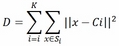
This equation denotes the optimization intrinsically done in the K-means algorithm: the centroids are chosen to minimize the intra-cluster distortion, that is, the sum of Euclidean norms of the distances between each input point and the centroid of the cluster to which the point is associated to. In other words, the algorithm tries to fit the best vectorial quantization.
The training phase of the K-means algorithm is also called Lloyd's algorithm, named after Stuart Lloyd, who first proposed the algorithm. It's an iterative algorithm composed of two phases iterated over and over till convergence (the distortion reaches a minimum). It's a variant of the generalized expectation-maximization (EM) algorithm as the first step creates a function for the expectation (E) of a score, and the maximization (M) step computes the parameters that maximize the score. (Note that in this formulation, we try to achieve the opposite, that is, the minimization of the distortion.) Here's its formulation:
- The expectation step: In this step, the points in the training set are assigned to the closest centroid:
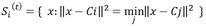
This step is also named assignment or vectorial quantization.
- The maximization step: The centroid of each cluster is moved to the middle of the cluster by averaging the points composing it:
This step is also named update step.
These two steps are performed till convergence (points are stable in their cluster), or till the algorithm reaches a preset number of iterations. Note that, per composition, the distortion cannot increase throughout the training phase (unlike Stochastic Gradient Descent-based methods); therefore, in this algorithm, the more iterations, the better the result.
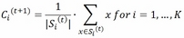
Let's now see how it looks like on a dummy two-dimensional dataset. We first create a set of 1,000 points concentrated in four locations symmetric with respect to the origin. Each cluster, per construction, has the same variance:
In:import matplotlib
import numpy as np
import pandas as pd
import matplotlib.pyplot as plt
%matplotlib inline

In:from sklearn.datasets.samples_generator import make_blobs


centers = [[1, 1], [1, -1], [-1, -1], [-1, 1]]
X, y = make_blobs(n_samples=1000, centers=centers,
                  cluster_std=0.5, random_state=101)
Let's now plot the dataset. To make things easier, we will color the clusters with different colors:
In:plt.scatter(X[:,0], X[:,1], c=y, edgecolors='none', alpha=0.9)
plt.show()
Let's now run K-means and inspect what's going on at each iteration. For this, we stop the iteration to 1, 2, 3, and 4 iterations and plot the points with their associated cluster (color-coded) as well as the centroid, distortion (in the title), and decision boundaries (also named Voronoi cells). The initial choice of the centroids is at random, that is, four training points are elected centroids in the first iteration during the expectation phase of the training:
In:pylab.rcParams['figure.figsize'] = (10.0, 8.0)

from sklearn.cluster import KMeans

for n_iter in range(1, 5):

    cls = KMeans(n_clusters=4, max_iter=n_iter, n_init=1,
                 init='random', random_state=101)
    cls.fit(X)


    # Plot the voronoi cells

    plt.subplot(2, 2, n_iter)
    h=0.02
    xx, yy = np.meshgrid(np.arange(-3, 3, h), np.arange(-3, 3, h))
    Z = cls.predict(np.c_[xx.ravel(),
        yy.ravel()]).reshape(xx.shape)
    plt.imshow(Z, interpolation='nearest', cmap=plt.cm.Accent,
               extent=(xx.min(), xx.max(), yy.min(), yy.max()),
               aspect='auto', origin='lower')


    plt.scatter(X[:,0], X[:,1], c=cls.labels_,
edgecolors='none', alpha=0.7)
    plt.scatter(cls.cluster_centers_[:,0],
                cls.cluster_centers_[:,1],
                marker='x', color='r', s=100, linewidths=4)
    plt.title("iter=%s, distortion=%s" %(n_iter,
                int(cls.inertia_)))

plt.show()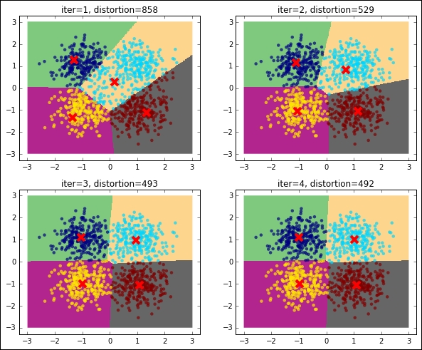
As you can see, the distortion is getting lower and lower as the number of iterations increases. For this dummy dataset, it seems that using a few iterations (five iterations), we've reached the convergence.
Finding the global minimum of the distortion in K-means is a NP-hard problem; moreover, exactly as with Stochastic Gradient Descent, this method is prone to converge to local minima especially if the number of dimensions is high. In order to avoid such behavior and limit the maximum number of iterations, you can use the following countermeasures:
- Run the algorithm multiple times using different initial conditions. In Scikit-learn, the
KMeansclass has then_initparameter that controls how many times the K-means algorithm will be run with different centroid seeds. At the end, the model that ensures the lower distortion is selected. If multiple cores are available, this process can be run in parallel by setting then_jobsparameter to the number of desired jobs to spin off. Note that the memory consumption is linearly dependent on the number of parallel jobs. - Prefer the k-means++ initialization (the
KMeansclass is the default) to the random choice of training points. K-means++ initialization selects points that are far among each other; this should ensure that the centroids are able to form clusters in uniform subspaces of the space. It's also proved that this fact ensures that it's more likely to find the best solution.
K-means relies on the assumptions that each cluster has a (hyper-) spherical shape, that is, it doesn't have an elongated shape (like an arrow), all the clusters have the same variance internally, and their size is comparable (or they are very far away).
All of these hypotheses can be guaranteed with a strong feature preprocessing step; PCA, KernelPCA, feature normalization, and sampling can be a good start.
Let's now see what happens when the assumptions behind K-means are not met:
In:pylab.rcParams['figure.figsize'] = (5.0, 10.0)
from sklearn.datasets import make_moons

# Oblong/elongated sets
X, _ = make_moons(n_samples=1000, noise=0.1, random_state=101)
cls = KMeans(n_clusters=2, random_state=101)
y_pred = cls.fit_predict(X)

plt.subplot(3, 1, 1)
plt.scatter(X[:, 0], X[:, 1], c=y_pred, edgecolors='none')
plt.scatter(cls.cluster_centers_[:,0], cls.cluster_centers_[:,1],
                marker='x', color='r', s=100, linewidths=4)
plt.title("Elongated clusters")

# Different variance between clusters
centers = [[-1, -1], [0, 0], [1, 1]]
X, _ = make_blobs(n_samples=1000, cluster_std=[0.1, 0.4, 0.1],
                  centers=centers, random_state=101)
cls = KMeans(n_clusters=3, random_state=101)
y_pred = cls.fit_predict(X)

plt.subplot(3, 1, 2)
plt.scatter(X[:, 0], X[:, 1], c=y_pred, edgecolors='none')
plt.scatter(cls.cluster_centers_[:,0], cls.cluster_centers_[:,1],
                marker='x', color='r', s=100, linewidths=4)
plt.title("Unequal Variance between clusters")

# Unevenly sized blobs
centers = [[-1, -1], [1, 1]]
centers.extend([[0,0]]*20)
X, _ = make_blobs(n_samples=1000, centers=centers,
                  cluster_std=0.28, random_state=101)
cls = KMeans(n_clusters=3, random_state=101)
y_pred = cls.fit_predict(X)

plt.subplot(3, 1, 3)
plt.scatter(X[:, 0], X[:, 1], c=y_pred, edgecolors='none')
plt.scatter(cls.cluster_centers_[:,0], cls.cluster_centers_[:,1],
                marker='x', color='r', s=100, linewidths=4)
plt.title("Unevenly Sized Blobs")

plt.show()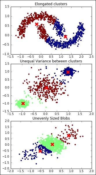
In all the preceding examples, the clustering operation is not perfect, outputting a wrong and unstable result.
So far, we've assumed to know exactly which is the exact K, the number of clusters that we're expecting to use in the clustering operation. Actually, in real-world problems, this is not always true. We often use an unsupervised learning method to discover the underlying structure of the data, including the number of clusters composing the dataset. Let's see what happens when we try to run K-means with a wrong K on a simple dummy dataset; we will try both a lower K and a higher one:
In:pylab.rcParams['figure.figsize'] = (10.0, 4.0)
X, _ = make_blobs(n_samples=1000, centers=3, random_state=101)

for K in [2, 3, 4]:
    cls = KMeans(n_clusters=K, random_state=101)
    y_pred = cls.fit_predict(X)

    plt.subplot(1, 3, K-1)
    plt.title("K-means, K=%s" % K)
    plt.scatter(X[:, 0], X[:, 1], c=y_pred, edgecolors='none')
    plt.scatter(cls.cluster_centers_[:,0], cls.cluster_centers_[:,1],
                marker='x', color='r', s=100, linewidths=4)

plt.show()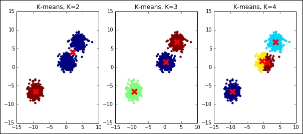
As you can see, the results are massively wrong in case the right K is not guessed, even for this simple dummy dataset. In the next section, we will explain some tricks to best select the K.
There are several methods to detect the best K if the assumptions behind K-means are met. Some of them are based on cross-validation and metrics on the output; they can be used on all clustering methods, but only when a ground truth is available (they're named supervised metrics). Some others are based on intrinsic parameters of the clustering algorithm and can be used independently by the presence or absence of the ground truth (also named unsupervised metrics). Unfortunately, none of them ensures 100% accuracy to find the correct result.
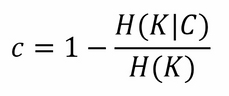
Supervised metrics require a ground truth (containing the true associations in sets) and they're usually combined with a gridsearch analysis to understand the best K. Some of these metrics are derived from equivalent classification ones, but they allow having a different number of unordered sets as predicted labels. The first one that we're going to see is named homogeneity; as you can expect, it gives a measure of how many of the predicted clusters contain just points of one class. It's a measure based on entropy, and it's the cluster equivalent of the precision in classification. It's a measure bound between 0 (worst) and 1 (best); its mathematical formulation is as follows:
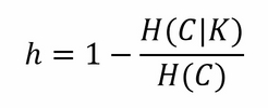
Here, H(C|K) is the conditional entropy of the class distribution given the proposed clustering assignment, and H(C) is the entropy of the classes. H(C|K) is maximal and equals H(C) when the clustering provides no new information; it is zero when each cluster contains only a member of a single class.
Connected to it, as in precision and recall for classification, there is the completeness score: it gives a measure about how much all members of a class are assigned to the same cluster. Even this one is bound between 0 (worst) and 1 (best), and its mathematical formulation is deeply based on entropy:
Here, H(K|C) is the conditional entropy of the proposed cluster distribution given the class, and H(K) is the entropy of the clusters.
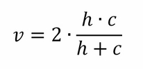
Finally, equivalent to the f1 score for the classification task, the V-measure is the harmonic mean of homogeneity and completeness:
Let's get back to the first dataset (four symmetric noisy clusters), and try to see how these scores operate and whether they are able to highlight the best K to use:
In:pylab.rcParams['figure.figsize'] = (6.0, 4.0)
from sklearn.metrics import homogeneity_completeness_v_measure


centers = [[1, 1], [1, -1], [-1, -1], [-1, 1]]
X, y = make_blobs(n_samples=1000, centers=centers,
                  cluster_std=0.5, random_state=101)

Ks = range(2, 10)
HCVs = []
for K in Ks:
    y_pred = KMeans(n_clusters=K, random_state=101).fit_predict(X)
    HCVs.append(homogeneity_completeness_v_measure(y, y_pred))

plt.plot(Ks, [el[0] for el in HCVs], 'r', label='Homogeneity')
plt.plot(Ks, [el[1] for el in HCVs], 'g', label='Completeness')
plt.plot(Ks, [el[2] for el in HCVs], 'b', label='V measure')
plt.ylim([0, 1])
plt.legend(loc=4)
plt.show()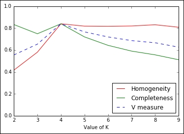
In the plot, initially (K<4) completeness is high, but homogeneity is low; for K>4, it is the opposite: homogeneity is high, but completeness is low. In both cases, the V-measure is low. For K=4, instead, all the measure reaches their maximum, indicating that's the best value for K, the number of clusters.
Beyond these metrics that are supervised, there are others named unsupervised that don't require a ground truth, but are just based on the learner itself.
The first that we're going to see in this section is the Elbow method, applied to the distortion. It's very easy and doesn't require any math: you just need to plot the distortion of many K-means models with different Ks, then select the one in which increasing K doesn't introduce much lower distortion in the solution. In Python, this is very simple to achieve:
In:Ks = range(2, 10)
Ds = []
for K in Ks:
    cls = KMeans(n_clusters=K, random_state=101)
    cls.fit(X)
    Ds.append(cls.inertia_)

plt.plot(Ks, Ds, 'o-')
plt.xlabel("Value of K")
plt.ylabel("Distortion")
plt.show()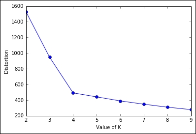
As you can expect, the distortion drops till K=4, then it decreases slowly. Here, the best-obtained K is 4.
Another unsupervised metric that we're going to see is the Silhouette. It's more complex, but also more powerful than the previous heuristics. At a very high level, it measures how close (similar) an observation is to the assigned cluster and how loosely (dissimilarly) it is matched to the data of nearby clusters. A Silhouette score of 1 indicates that all the data is in the best cluster, and -1 indicates a completely wrong cluster result. To obtain such a measure using Python code is very easy, thanks to the Scikit-learn implementation:
In:from sklearn.metrics import silhouette_score

Ks = range(2, 10)
Ds = []
for K in Ks:
    cls = KMeans(n_clusters=K, random_state=101)
    Ds.append(silhouette_score(X, cls.fit_predict(X)))

plt.plot(Ks, Ds, 'o-')
plt.xlabel("Value of K")
plt.ylabel("Silhouette score")
plt.show()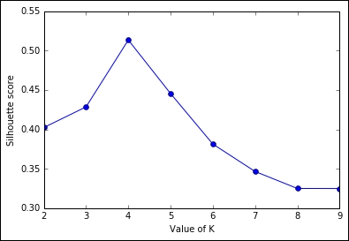
Even in this case, we've arrived at the same conclusion: the best value for K is 4 as the silhouette score is much lower with a lower and higher K.
Let's now test the scalability of K-means. From the website of UCI, we've selected an appropriate dataset for this task: the US Census 1990 Data. This dataset contains almost 2.5 million observations and 68 categorical (but already number-encoded) attributes. There is no missing data and the file is in the CSV format. Each observation contains the ID of the individual (to be removed before the clustering) and other information about gender, income, marital status, work, and so on.
Note
Further information about the dataset can be found at http://archive.ics.uci.edu/ml/datasets/US+Census+Data+%281990%29 or in the paper published in The Journal of Machine Learning Research by Meek, Thiesson, and Heckerman (2001) entitled The Learning Curve Method Applied to Clustering.
As the first thing to be done, you have to download the file containing the dataset and store it in a temporary directory. Note that it's 345MB in size, therefore its download might require a long time on slow connections:
In:import urllib
import os.path

url = "http://archive.ics.uci.edu/ml/machine-learning-databases/census1990-mld/USCensus1990.data.txt"
census_csv_file = "/tmp/USCensus1990.data.txt"

import os.path
if not os.path.exists(census_csv_file):
    testfile = urllib.URLopener()
    testfile.retrieve(url, census_csv_file)
Now, let's run some tests clocking the times needed to train a K-means learner with K equal to 4, 8, and 12, and with a dataset containing 20K, 200K, and 0.5M observations. As we don't want to saturate the memory of the machine, consequently we will just read the first 500K lines and drop the column containing the identifier of the user. Finally, let's plot the training times for a complete performance evaluation:
In:piece_of_dataset = pd.read_csv(census_csv_file, iterator=True).get_chunk(500000).drop('caseid', axis=1).as_matrix()

time_results = {4: [], 8:[], 12:[]}
dataset_sizes = [20000, 200000, 500000]


for dataset_size in dataset_sizes:
    print "Dataset size:", dataset_size
    X = piece_of_dataset[:dataset_size,:]

    for K in [4, 8, 12]:
        print "K:", K
        cls = KMeans(K, random_state=101)
        timeit = %timeit -o -n1 -r1 cls.fit(X)

        time_results[K].append(timeit.best)

plt.plot(dataset_sizes, time_results[4], 'r', label='K=4')
plt.plot(dataset_sizes, time_results[8], 'g', label='K=8')
plt.plot(dataset_sizes, time_results[12], 'b', label='K=12')

plt.xlabel("Training set size")
plt.ylabel("Training time")
plt.legend(loc=0)
plt.show()

Out:Dataset size: 20000
K: 4
1 loops, best of 1: 478 ms per loop
K: 8
1 loops, best of 1: 1.22 s per loop
K: 12
1 loops, best of 1: 1.76 s per loop
Dataset size: 200000
K: 4
1 loops, best of 1: 6.35 s per loop
K: 8
1 loops, best of 1: 10.5 s per loop
K: 12
1 loops, best of 1: 17.7 s per loop
Dataset size: 500000
K: 4
1 loops, best of 1: 13.4 s per loop
K: 8
1 loops, best of 1: 48.6 s per loop
K: 12
1 loops, best of 1: 1min 5s per loop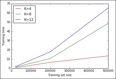
It seems clear that, given the plot and actual timings, the training time increases linearly with K and the training set size, but for large Ks and training sizes, such a relation becomes nonlinear. Doing an exhaustive search with the whole training set for many Ks does not seem scalable.
Fortunately, there's an online version of K-means based on mini-batches, already implemented in Scikit-learn and named MiniBatchKMeans. Let's try it on the slowest case of the previous cell, that is, with K=12. With the classic K-means, the training on 500,000 samples (circa 20% of the full dataset) took more than a minute; let's see the performance of the online mini-batch version, setting the batch size to 1,000 and importing chunks of 50,000 observations from the dataset. As an output, we plot the training time versus the number of chunks already passed thought the training phase:
In:from sklearn.cluster import MiniBatchKMeans
import time

cls = MiniBatchKMeans(12, batch_size=1000, random_state=101)
ts = []

tik = time.time()
for chunk in pd.read_csv(census_csv_file, chunksize=50000):
    cls.partial_fit(chunk.drop('caseid', axis=1))
    ts.append(time.time()-tik)

plt.plot(range(len(ts)), ts)
plt.xlabel('Training batches')
plt.ylabel('time [s]')

plt.show()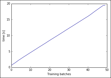
Training time is linear for each chunk, performing the clustering on the full 2.5 million observations dataset in nearly 20 seconds. With this implementation, we can run a full search to select the best K using the elbow method on the distortion. Let's do a gridsearch, with K spanning from 4 to 12, and plot the distortion:
In:Ks = list(range(4, 13))
ds = []

for K in Ks:
    cls = MiniBatchKMeans(K, batch_size=1000, random_state=101)

    for chunk in pd.read_csv(census_csv_file, chunksize=50000):
        cls.partial_fit(chunk.drop('caseid', axis=1))
    ds.append(cls.inertia_)

plt.plot(Ks, ds)
plt.xlabel('Value of K')
plt.ylabel('Distortion')

plt.show()

Out: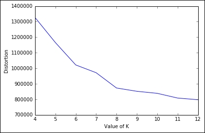
From the plot, the elbow seems in correspondence of K=8. Beyond the value, we would like to point out that in less than a couple of minutes, we've been able to perform this massive operation on a large dataset, thanks to the batch implementation; therefore remember never to use the plain vanilla K-means if the dataset is getting big.