In order to use the Spark functionalities (or pySpark, containing the Python APIs of Spark), we need to instantiate a special object named SparkContext. It tells Spark how to access the cluster and contains some application-specific parameters. In the IPython Notebook provided in the virtual machine, this variable is already available and named sc (it's the default option when an IPython Notebook is started); let's now see what it contains.

First, open a new IPython Notebook; when it's ready to be used, type the following in the first cell:

In:sc._conf.getAll()

Out:[(u'spark.rdd.compress', u'True'),
 (u'spark.master', u'yarn-client'),
 (u'spark.serializer.objectStreamReset', u'100'),
 (u'spark.yarn.isPython', u'true'),
 (u'spark.submit.deployMode', u'client'),
 (u'spark.executor.cores', u'2'),
 (u'spark.app.name', u'PySparkShell')]

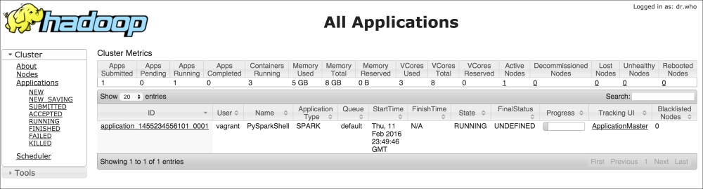
It contains multiple information: the most important is the spark.master, in this case set as a client in YARN, spark.executor.cores set to two as the number of CPUs of the virtual machine, and spark.app.name, the name of the application. The name of the app is particularly useful when the (YARN) cluster is shared; going to ht.0.0.1:8088, it is possible to check the state of the application:

The data model used by Spark is named Resilient Distributed Dataset (RDD), which is a distributed collection of elements that can be processed in parallel. An RDD can be created from an existing collection (a Python list, for example) or from an external dataset, stored as a file on the local machine, HDFS, or other sources.

Let's now create an RDD containing integers from 0 to 9. To do so, we can use the parallelize method provided by the SparkContext object:

In:numbers = range(10)
numbers_rdd = sc.parallelize(numbers)

numbers_rdd

Out:ParallelCollectionRDD[1] at parallelize at PythonRDD.scala:423

As you can see, you can't simply print the RDD content as it's split into multiple partitions (and distributed in the cluster). The default number of partitions is twice the number of CPUs (so, it's four in the provided VM), but it can be set manually using the second argument of the parallelize method.

To print out the data contained in the RDD, you should call the collect method. Note that this operation, while run on a cluster, collects all the data on the node; therefore, the node should have enough memory to contain it all:

In:numbers_rdd.collect()

Out:[0, 1, 2, 3, 4, 5, 6, 7, 8, 9]

To obtain just a partial peek, use the take method indicating how many elements you'd want to see. Note that as it's a distributed dataset, it's not guaranteed that elements are in the same order as when we inserted it:

In:numbers_rdd.take()

Out:[0, 1, 2, 3]

To read a text file, we can use the textFile method provided by the Spark Context. It allows reading both HDFS files and local files, and it splits the text on the newline characters; therefore, the first element of the RDD is the first line of the text file (using the first method). Note that if you're using a local path, all the nodes composing the cluster should access the same file through the same path:

In:sc.textFile("hdfs:///datasets/hadoop_git_readme.txt").first()

Out:u'For the latest information about Hadoop, please visit our website at:'

In:sc.textFile("file:///home/vagrant/datasets/hadoop_git_readme.txt").first()

Out:u'For the latest information about Hadoop, please visit our website at:'

To save the content of an RDD on disk, you can use the saveAsTextFile method provided by the RDD. Here, you can use multiple destinations; in this example, let's save it in HDFS and then list the content of the output:

In:numbers_rdd.saveAsTextFile("hdfs:///tmp/numbers_1_10.txt")

In:!hdfs dfs -ls /tmp/numbers_1_10.txt

Out:Found 5 items
-rw-r--r--   1 vagrant supergroup          0 2016-02-12 14:18 /tmp/numbers_1_10.txt/_SUCCESS
-rw-r--r--   1 vagrant supergroup          4 2016-02-12 14:18 /tmp/numbers_1_10.txt/part-00000
-rw-r--r--   1 vagrant supergroup          4 2016-02-12 14:18 /tmp/numbers_1_10.txt/part-00001
-rw-r--r--   1 vagrant supergroup          4 2016-02-12 14:18 /tmp/numbers_1_10.txt/part-00002
-rw-r--r--   1 vagrant supergroup          8 2016-02-12 14:18 /tmp/numbers_1_10.txt/part-00003

Spark writes one file for each partition, exactly as MapReduce, writing one file for each reducer. This way speeds up the saving time as each partition is saved independently, but on a 1-node cluster, it makes things harder to read.

Can we take all the partitions to 1 before writing the file or, generically, can we lower the number of partitions in an RDD? The answer is yes, through the coalesce method provided by the RDD, passing the number of partitions we'd want to have as an argument. Passing 1 forces the RDD to be in a standalone partition and, when saved, produces just one output file. Note that this happens even when saving on the local filesystem: a file is created for each partition. Mind that doing so on a cluster environment composed by multiple nodes won't ensure that all the nodes see the same output files:

In:
numbers_rdd.coalesce(1) 
.saveAsTextFile("hdfs:///tmp/numbers_1_10_one_file.txt")

In : !hdfs dfs -ls /tmp/numbers_1_10_one_file.txt

Out:Found 2 items
-rw-r--r--   1 vagrant supergroup          0 2016-02-12 14:20 /tmp/numbers_1_10_one_file.txt/_SUCCESS
-rw-r--r--   1 vagrant supergroup         20 2016-02-12 14:20 /tmp/numbers_1_10_one_file.txt/part-00000

In:!hdfs dfs -cat /tmp/numbers_1_10_one_file.txt/part-00000

Out:0
1
2
3
4
5
6
7
8
9

In:numbers_rdd.saveAsTextFile("file:///tmp/numbers_1_10.txt")

In:!ls /tmp/numbers_1_10.txt

Out:part-00000  part-00001    part-00002  part-00003    _SUCCESS

An RDD supports just two types of operations:

Typical Spark programs are a chain of transformations with an action at the end. By default, all the transformations on the RDD are executed each time you run an action (that is, the intermediate state after each transformer is not saved). However, you can override this behavior using the persist method (on the RDD) whenever you want to cache the value of the transformed elements. The persist method allows both memory and disk persistency.

In the next example, we will square all the values contained in an RDD and then sum them up; this algorithm can be executed through a mapper (square elements) followed by a reducer (summing up the array). According to Spark, the map method is a transformer as it just transforms the data element by element; reduce is an action as it creates a value out of all the elements together.

Let's approach this problem step by step to see the multiple ways in which we can operate. First, start with the mapping: we first define a function that returns the square of the input argument, then we pass this function to the map method in the RDD, and finally we collect the elements in the RDD:

In:
def sq(x):
    return x**2

numbers_rdd.map(sq).collect()

Out:[0, 1, 4, 9, 16, 25, 36, 49, 64, 81]

Although the output is correct, the sq function is taking a lot of space; we can rewrite the transformation more concisely, thanks to Python's lambda expression, in this way:

In:numbers_rdd.map(lambda x: x**2).collect()

Out:[0, 1, 4, 9, 16, 25, 36, 49, 64, 81]

Remember: why did we need to call collect to print the values in the transformed RDD? This is because the map method will not spring to action, but will be just lazily evaluated. The reduce method, on the other hand, is an action; therefore, adding the reduce step to the previous RDD should output a value. As for map, reduce takes as an argument a function that should have two arguments (left value and right value) and should return a value. Even in this case, it can be a verbose function defined with def or a lambda function:

In:numbers_rdd.map(lambda x: x**2).reduce(lambda a,b: a+b)

Out:285

To make it even simpler, we can use the sum action instead of the reducer:

In:numbers_rdd.map(lambda x: x**2).sum()

Out:285

So far, we've shown a very simple example of pySpark. Think about what's going on under the hood: the dataset is first loaded and partitioned across the cluster, then the mapping operation is run on the distributed environment, and then all the partitions are collapsed together to generate the result (sum or reduce), which is finally printed on the IPython Notebook. A huge task, yet made super simple by pySpark.

Let's now advance one step and introduce the key-value pairs; although RDDs can contain any kind of object (we've seen integers and lines of text so far), a few operations can be made when the elements are tuples composed by two elements: key and value.

To show an example, let's now first group the numbers in the RDD in odds and evens and then compute the sum of the two groups separately. As for the MapReduce model, it would be nice to map each number with a key (odd or even) and then, for each key, reduce using a sum operation.

We can start with the map operation: let's first create a function that tags the numbers, outputting even if the argument number is even, odd otherwise. Then, create a key-value mapping that creates a key-value pair for each number, where the key is the tag and the value is the number itself:

In:
def tag(x):
    return "even" if x%2==0 else "odd"


numbers_rdd.map(lambda x: (tag(x), x) ).collect()

Out:[('even', 0),
 ('odd', 1),
 ('even', 2),
 ('odd', 3),
 ('even', 4),
 ('odd', 5),
 ('even', 6),
 ('odd', 7),
 ('even', 8),
 ('odd', 9)]

To reduce each key separately, we can now use the reduceByKey method (which is not a Spark action). As an argument, we should pass the function that we should apply to all the values of each key; in this case, we will sum up all of them. Finally, we should call the collect method to print the results:

In:
numbers_rdd.map(lambda x: (tag(x), x) ) 
.reduceByKey(lambda a,b: a+b).collect()

Out:[('even', 20), ('odd', 25)]

Now, let's list some of the most important methods available in Spark; it's not an exhaustive guide, but just includes the most used ones.

We start with transformations; they can be applied to an RDD and they produce an RDD:

Now, let's overview what are the most popular actions available in pySpark. Note that actions trigger the processing of the RDD through all the transformers in the chain:

There are also a few methods that are neither transformers nor actions:

Let's now try to replicate the examples that we've seen in the section about MapReduce with Hadoop. With Spark, the algorithm should be as follows:

In:
def emit_feats(line):
    return [("chars", len(line)), 
            ("words", len(line.split())), 
            ("lines", 1)]

print (sc.textFile("/datasets/hadoop_git_readme.txt")
 .flatMap(emit_feats)
 .reduceByKey(lambda a,b: a+b)
 .collectAsMap())

Out:{'chars': 1335, 'lines': 31, 'words': 179}

We can immediately note the enormous speed of this method compared to the MapReduce implementation. This is because all of the dataset is stored in-memory and not in HDFS. Secondly, this is a pure Python implementation and we don't need to call external command lines or libraries—pySpark is self-contained.

Let's now work on the example on the larger file, containing the Shakespeare texts, to extract the most popular word. In the Hadoop MapReduce implementation, it takes two map-reduce steps and therefore four write/read on HDFS. In pySpark, we can do all this in an RDD:

In:import re
WORD_RE = re.compile(r"[w']+")

print (sc.textFile("/datasets/shakespeare_all.txt")
 .flatMap(lambda line: WORD_RE.findall(line))
 .map(lambda word: (word.lower(), 1))
 .reduceByKey(lambda a,b: a+b)
 .map(lambda (k,v): (v,k))
 .takeOrdered(1, key = lambda x: -x[0]))

Out:[(27801, u'the')]

The results are the same that we had using Hadoop and MapReduce, but in this case, the computation takes far less time. We can actually further improve the solution, collapsing the second and third steps together (flatMap-ing a key-value pair for each word, where the key is the lowercased word and value is the number of occurrences) and the fifth and sixth steps together (taking the first element and ordering the elements in the RDD by their value, that is, the second element of the pair):

In:
print (sc.textFile("/datasets/shakespeare_all.txt")
 .flatMap(lambda line: [(word.lower(), 1) for word in WORD_RE.findall(line)])
 .reduceByKey(lambda a,b: a+b)
 .takeOrdered(1, key = lambda x: -x[1]))

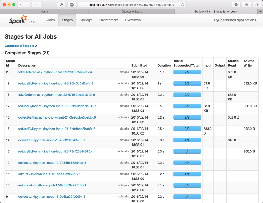
Out:[(u'the', 27801)]

To check the state of the processing, you can use the Spark UI: it's a graphical interface that shows the jobs run by Spark step-by-step. To access the UI, you should first figure out what's the name of the pySpark IPython application, searching in the bash shell where you've launched the notebook by its name (typically, it is in the form application_<number>_<number>), and then point your browser to the page: http://localhost:8088/proxy/application_<number>_<number>

The result is similar to the one in the following image. It contains all the jobs run in spark (as IPython Notebook cells), and you can also visualize the execution plan as a directed acyclic graph (DAG):