One of the standards for file formats is CSV. In this section, we will walk through the process of reading a CSV and adjusting the dataset to arrive at some conclusions about the data. The data I am using is from the Heating System Choice in California Houses dataset, found at https://vincentarelbundock.github.io/Rdatasets/datasets.html:

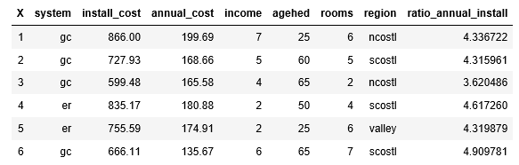
#read in the CSV file as available on the site
heating <- read.csv(file="Documents/heating.csv", header=TRUE, sep=",")
# make sure the data is laid out the way we expect
head(heating)  

The data appears to be as expected; however, a number of the columns have acronym names and are somewhat duplicated. Let us change the names of interest that we want to be more readable and remove the extras we are not going to use:

# change the column names to be more readable
colnames(heating)[colnames(heating)=="depvar"] <- "system"
colnames(heating)[colnames(heating)=="ic.gc"] <- "install_cost"
colnames(heating)[colnames(heating)=="oc.gc"] <- "annual_cost"
colnames(heating)[colnames(heating)=="pb.gc"] <- "ratio_annual_install"

# remove columns which are not used
heating$idcase <- NULL
heating$ic.gr <- NULL
heating$ic.ec <- NULL
heating$ic.hp <- NULL
heating$ic.er <- NULL
heating$oc.gr <- NULL
heating$oc.ec <- NULL
heating$oc.hp <- NULL
heating$oc.er <- NULL
heating$pb.gr <- NULL
heating$pb.ec <- NULL
heating$pb.er <- NULL
heating$pb.hp <- NULL

# check the data layout again now that we have made changes
head(heating)  

Now that we have a tighter dataset, let us start to look over the data:

# get rough statistics on the data
summary(heating)  

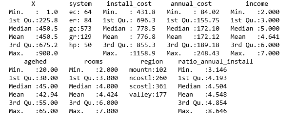
Some points pop out from the summary:

• There are five different types of heating systems, gas cooling being most prevalent
• Costs vary much more than expected
• The data covers four large regions of California
• The ration of the annual cost versus the initial cost varies much more than expected

It is not obvious what the data relationships might be, but we can use the R plot() function to provide a quick snapshot that shows anything significant:

plot(heating)  

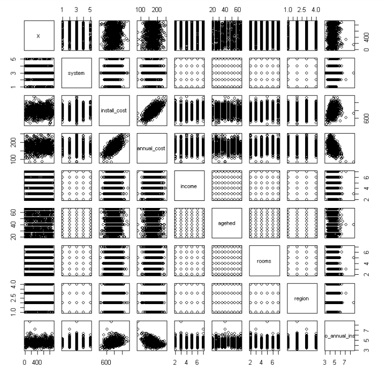
Again, several interesting facts jump out:

• The initial cost varies widely within the type of system
• The annual cost varies within the type of system as well
• Costs vary widely within the ranges of customer income, age, number of rooms in the house, and region

The only direct relationship between variables appears to be the initial cost of system and the annual cost. With covariance, we are looking for a measure of how much two variables change in relation to each other. If we run a covariance between the install and annual cost, we get:

cov(heating$install_cost, heating$annual_cost) 
2131  

I am not sure I have seen a higher covariance result.