In Python, we have very similar steps for producing nearest neighbor estimation.
First, we import the packages to be used:

from sklearn.neighbors import NearestNeighbors 
import numpy as np 
import pandas as pd 

Numpy and pandas are standards. Nearest neighbors is one of the sklearn features.
Now, we load in our housing data:

housing = pd.read_csv("http://archive.ics.uci.edu/ml/machine-learning-databases/housing/housing.data",
                       header=None, sep='s+') 
housing.columns = ["CRIM", "ZN", "INDUS", "CHAS", "NOX", "RM", "AGE",  
"DIS", "RAD", "TAX", "PRATIO",  
"B", "LSTAT", "MDEV"] 
housing.head(5) 

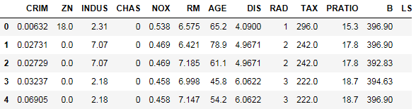
The same data that we saw previously in R.
Let us see how big it is:

len(housing) 
506 

And break up the data into a training and testing set:

mask = np.random.rand(len(housing)) < 0.8 
training = housing[mask] 
testing = housing[~mask] 
len(training) 
417 
len(testing) 
89 

Find the nearest neighbors:

nbrs = NearestNeighbors().fit(housing) 

Display their indices and distances. Indices are varying quite a lot. Distances seem to be in bands:

distances, indices = nbrs.kneighbors(housing) 
indices 
array([[  0, 241,  62,  81,   6], 
       [  1,  47,  49,  87,   2], 
       [  2,  85,  87,  84,   5], 
       ...,  
       [503, 504, 219,  88, 217], 
       [504, 503, 219,  88, 217], 
       [505, 502, 504, 503,  91]], dtype=int32) 
distances 
array([[  0.        ,  16.5628085 , 17.09498324,18.40127391, 
         19.10555821], 
       [  0.        ,  16.18433277, 20.59837827, 22.95753545, 
         23.05885288] 
       [  0.        ,  11.44014392, 15.34074743, 19.2322435 , 
         21.73264817], 
       ...,  
       [  0.        ,   4.38093898,  9.44318468, 10.79865973, 
         11.95458848], 
       [  0.        ,   4.38093898,  8.88725757, 10.88003717, 
         11.15236419], 
       [  0.        ,   9.69512304, 13.73766871, 15.93946676, 
         15.94577477]]) 

Build a nearest neighbors model from the training set:

from sklearn.neighbors import KNeighborsRegressor 
knn = KNeighborsRegressor(n_neighbors=5) 
x_columns = ["CRIM", "ZN", "INDUS", "CHAS", "NOX", "RM", "AGE", "DIS", "RAD", "TAX", "PRATIO", "B", "LSTAT"] 
y_column = ["MDEV"] 
knn.fit(training[x_columns], training[y_column]) 
KNeighborsRegressor(algorithm='auto', leaf_size=30, metric='minkowski', 
          metric_params=None, n_jobs=1, n_neighbors=5, p=2, 
          weights='uniform') 

It is interesting that with Python we do not have to store models off separately. Methods are stateful.

Make our predictions:

predictions = knn.predict(testing[x_columns])
predictions
array([[ 20.62],
       [ 21.18],
       [ 23.96],
       [ 17.14],
       [ 17.24],
       [ 18.68],
       [ 28.88],

Determine how well we have predicted the housing price:

columns = ["testing","prediction","diff"] 
index = range(len(testing)) 
results = pd.DataFrame(index=index, columns=columns) 
 
results['prediction'] = predictions 
 
results = results.reset_index(drop=True) 
testing = testing.reset_index(drop=True) 
results['testing'] = testing["MDEV"] 
 
results['diff'] = results['testing'] - results['prediction'] 
results['pct'] = results['diff'] / results['testing'] 
results.mean() 
testing       22.159551 
prediction    22.931011 
diff          -0.771461 
pct           -0.099104 

We have a mean difference of ¾ versus an average value of 22. This should mean an average percent difference of about 3%, but the average percentage difference calculated is close to 10%. So, we are not estimating well under Python.