We can perform the same analysis using R in a notebook. The functions are different for the different language, but the functionality is very close.
We use the same algorithm:
- Load the dataset
- Split the dataset into training and testing partitions
- Develop a model based on the training partition
- Use the model to predict from the testing partition
- Compare predicted versus actual testing
The coding is as follows:
#load in the data set from uci.edu (slightly different from other housing model)
housing <- read.table("http://archive.ics.uci.edu/ml/machine-learning-databases/housing/housing.data")

#assign column names
colnames(housing) <- c("CRIM", "ZN", "INDUS", "CHAS", "NOX",
                  "RM", "AGE", "DIS", "RAD", "TAX", "PRATIO",
                  "B", "LSTAT", "MDEV")
#make sure we have the right data being loaded
summary(housing)
      CRIM                ZN             INDUS            CHAS
 Min.   : 0.00632   Min.   :  0.00   Min.   : 0.46   Min.   :0.00000
 1st Qu.: 0.08204   1st Qu.:  0.00   1st Qu.: 5.19   1st Qu.:0.00000
 Median : 0.25651   Median :  0.00   Median : 9.69   Median :0.00000
 Mean   : 3.61352   Mean   : 11.36   Mean   :11.14   Mean   :0.06917
 3rd Qu.: 3.67708   3rd Qu.: 12.50   3rd Qu.:18.10   3rd Qu.:0.00000
 Max.   :88.97620   Max.   :100.00   Max.   :27.74   Max.   :1.00000
      NOX               RM             AGE              DIS
 Min.   :0.3850   Min.   :3.561   Min.   :  2.90   Min.   : 1.130
 1st Qu.:0.4490   1st Qu.:5.886   1st Qu.: 45.02   1st Qu.: 2.100
 Median :0.5380   Median :6.208   Median : 77.50   Median : 3.207
 Mean   :0.5547   Mean   :6.285   Mean   : 68.57   Mean   : 3.795
 3rd Qu.:0.6240   3rd Qu.:6.623   3rd Qu.: 94.08   3rd Qu.: 5.188
 Max.   :0.8710   Max.   :8.780   Max.   :100.00   Max.   :12.127
...
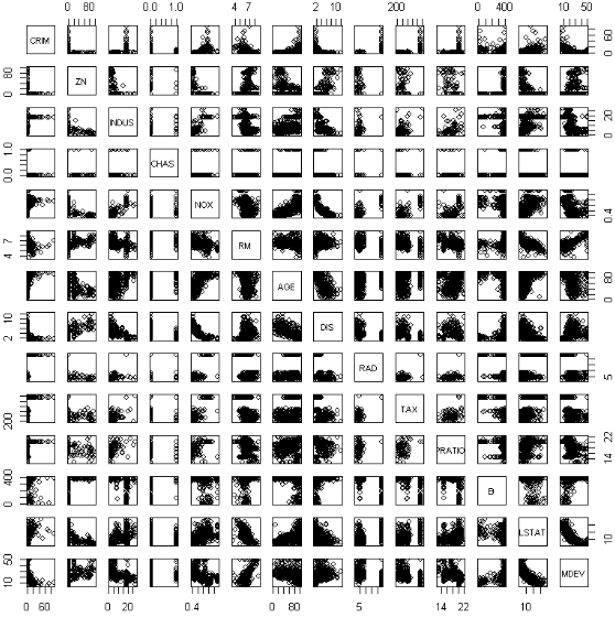
housing <- housing[order(housing$MDEV),]

#check if there are any relationships between the data items
plot(housing)
The data display, shown as follows, plots every variable against every other variable in the dataset. I am looking to see if there are any nice 45 degree 'lines' showing great symmetry between the variables, with the idea that maybe we should remove one as the other suffices as a contributing factor. The interesting items are:
- CHAS: Charles River access, but that is a binary value.
- LSTAT (lower status population) and MDEV (price) have an inverse relationship—but price will not be a factor.
- NOX (smog) and DIST (distance to work) have an inverse relationship. I think we want that.
- Otherwise, there doesn't appear to be any relationship between the data items:
We go about forcing the seed, as before, to be able to reproduce results. We then split the data into training and testing partitions made with the createDataPartitions function. We can then train our model and test the resultant model for validation:
#force the random seed so we can reproduce results
set.seed(133)

#caret package has function to partition data set
library(caret)
trainingIndices <- createDataPartition(housing$MDEV, p=0.75, list=FALSE)
#break out the training vs testing data sets
housingTraining <- housing[trainingIndices,]
housingTesting <- housing[-trainingIndices,]
#note their sizes
nrow(housingTraining)
nrow(housingTesting)
#note there may be warning messages to update packages
381
125

#build a linear model
linearModel <- lm(MDEV ~ CRIM + ZN + INDUS + CHAS + NOX + RM + AGE +
                 DIS + RAD + TAX + PRATIO + B + LSTAT, data=housingTraining)
summary(linearModel)
Call:
lm(formula = MDEV ~ CRIM + ZN + INDUS + CHAS + NOX + RM + AGE +
    DIS + RAD + TAX + PRATIO + B + LSTAT, data = housingTraining)

Residuals:
     Min       1Q   Median       3Q      Max
-15.8448  -2.7961  -0.5602   2.0667  25.2312

Coefficients:
              Estimate Std. Error t value Pr(>|t|)
(Intercept)  36.636334   5.929753   6.178 1.72e-09 ***
CRIM         -0.134361   0.039634  -3.390 0.000775 ***
ZN            0.041861   0.016379   2.556 0.010997 *
INDUS         0.029561   0.068790   0.430 0.667640
CHAS          3.046626   1.008721   3.020 0.002702 **
NOX         -17.620245   4.610893  -3.821 0.000156 ***
RM            3.777475   0.484884   7.790 6.92e-14 ***
AGE           0.003492   0.016413   0.213 0.831648
DIS          -1.390157   0.235793  -5.896 8.47e-09 ***
RAD           0.309546   0.078496   3.943 9.62e-05 ***
TAX          -0.012216   0.004323  -2.826 0.004969 **
PRATIO       -0.998417   0.155341  -6.427 4.04e-10 ***
B             0.009745   0.003300   2.953 0.003350 **
LSTAT        -0.518531   0.060614  -8.555 3.26e-16 ***
---
Signif. codes:  0 '***' 0.001 '**' 0.01 '*' 0.05 '.' 0.1 ' ' 1

Residual standard error: 4.867 on 367 degrees of freedom
Multiple R-squared:  0.7327,  Adjusted R-squared:  0.7233
F-statistic:  77.4 on 13 and 367 DF,  p-value: < 2.2e-16
It is interesting that this model also picked up on a high premium for Charles River views affecting the price. Also, like that, this model provides p-value (good confidence in the model):
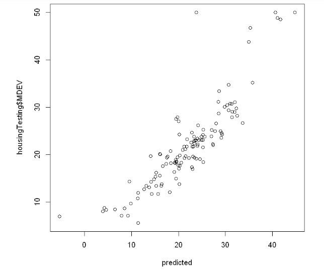
# now that we have a model, make a prediction
predicted <- predict(linearModel,newdata=housingTesting)
summary(predicted)

#visually compare prediction to actual
plot(predicted, housingTesting$MDEV)
It looks like a pretty good correlation, very close to a 45 degree mapping. The exception is that the predicted values are a little higher than actuals: