Given the preceding results it appears that people mostly only vote in a positive manner. We can look to see if there is a relationship between how many votes a company has received and their rating.

First, we accumulate the dataset using the following script, extracting the number of votes and rating for each firm:

#determine relationship between number of reviews and star rating
import pandas as pd
from pandas import DataFrame as df  
import numpy as np  

dfr2 = pd.DataFrame(columns=['reviews', 'rating'])
mynparray = dfr2.values

for line in lines:
    line = unicode(line, errors='ignore')
    obj = json.loads(line)
    reviews = int(obj['review_count'])
    rating = float(obj['stars'])
    arow = [reviews,rating]
    mynparray = np.vstack((mynparray,arow)) 

dfr2 = df(mynparray)
print (len(dfr2))  

This coding just builds the data frame with our two variables. We are using NumPy as it more easily adds a row to a data frame. Once we are done with all records we convert the NumPy data frame back to a pandas data frame.

The column names have been lost in the translation, so we put those back in and draw some summary statistics:

dfr2.columns = ['reviews', 'rating']
dfr2.describe()

In the output shown as follows we see the layout of the reviews and rating data we have collected. Yelp has not constrained its data entry for this dataset. There should 5 unique values for rating:

Next, we plot the data for a visual clue to the relationship, using the following:

#import matplotlib.pyplot as plt
dfr2.plot(kind='scatter', x='rating', y='reviews')
plt.show()  

So, the data after all, appears to have a clear Poisson distribution as compared to the earlier business_rating histogram.

Next, we compute the regression parameters:

#compute regression
import statsmodels.formula.api as smf

# create a fitted model in one line
lm = smf.ols(formula='rating ~ reviews', data=dfr2).fit()

# print the coefficients
lm.params  

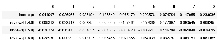
We computed intercepts for all rating values. I had expected a single value.

Now, we determine the range of the observed data using the following:

#min, max observed values
X_new = pd.DataFrame({'reviews': [dfr2.reviews.min(), dfr2.reviews.max()]})
X_new.head()  

So, as we guessed earlier, some businesses have a very large number of reviews.

Now, we can make predictions based on the extent data points:
#make corresponding predictions
preds = lm.predict(X_new)
preds  

We are seeing a much bigger range of predicted values than expected. Plot out the observed and predicted data:

# first, plot the observed data
dfr2.plot(kind='scatter', x='reviews', y='rating')

# then, plot the least squares line
plt.plot(X_new, preds, c='red', linewidth=2)
plt.show()  

In the plot displayed as follows, there does not appear to be a relationship between the number of reviews and the review score for a firm. It appears to be a numbers game—if you get people to review your firm, on average they will give you a high score.

There does not appear to be a relationship between the number of reviews and the review score for a firm.