The tidyr package is available to clean up/tidy your dataset. The use of tidyr is to rearrange your data so that:

• Each column is a variable
• Each row is an observation

When your data is arranged in this manner, it becomes much easier to analyze. There are many datasets published that mix columns and rows with values. You then must adjust them accordingly if you use the data in situ.

tidyr provides three functions for cleaning up your data:

• gather
• separate
• spread

The gather() function takes your data and arranges the data into key-value pairs, much like the Hadoop database model. Let's use the standard example of stock prices for a date using the following:

library(tidyr)
stocks <- data_frame(
  time = as.Date('2017-08-05') + 0:9,
  X = rnorm(10, 20, 1), #how many numbers, mean, std dev
  Y = rnorm(10, 20, 2),
  Z = rnorm(10, 20, 4)
)

This will generate data that looks like this:

Every row has a timestamp and the prices of the three stocks at that time.

We first use gather() to split out key-value pairs for the stocks. The gather() function is called with the data frame that it will work with, the output column names, and the columns to ignore (-time). So we get a row with the distinct time, stock, and prices using the following:

stocksg <- gather(stocks, stock, price, -time)
head(stocksg)  

This will generate the following head() display:

The separate() function is used to split apart values that are in the same entry points.

We will use Dow Jones Index history about industrial prices from UCI (https://archive.ics.uci.edu/ml/datasets/Dow+Jones+Index):

dji <- read.csv("Documents/dow_jones_index.data")
dj <- dji[,c("stock","date","close")]
summary(dj)
head(dj)

So, we have the date already gathered to start with (if we had disorganized data to start with, we would have used gather to organize it up to this point).

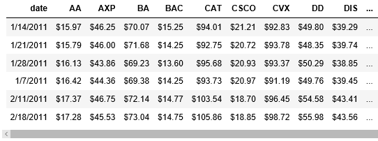
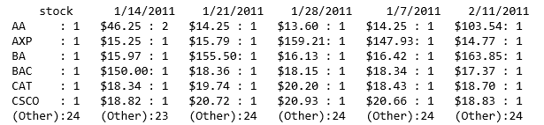
The spread() function will take the key-value pairs (from the gather() function) and separate out the values into multiple columns. We call spread() using the data frame containing our source date, the values to use for our columns, and the data points for each date/column. Continuing with our example, we can spread out all of the securities by date using:

prices <- dj %>% spread(stock, close)
summary(prices)
head(prices)  

This results in the following summary display (shortened to just the first few securities):

It also results in the following head display, showing the prices of all the securities by date:

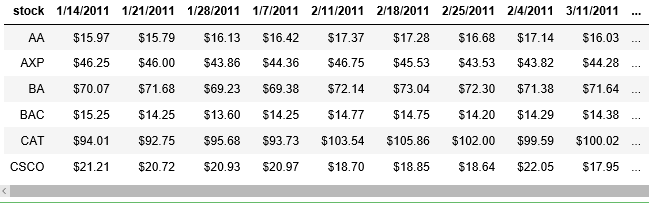
We can also similarly reorganize the data by listing all prices for a stock per row using:

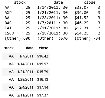
times <- dj %>% spread(date, close)
summary(times)
head(times)  

Here, our row driver is the stock, the column heading is the date value, and the data point for each stock/date is the closing price of the security on that date.

From the summary (abbreviated), we can see the following:

The following is the head sample showing the data in our desired format: