Spark exposes many SQL-like actions that can be taken upon a data frame. For example, we could load a data frame with product sales information in a CSV file:

from pyspark.sql import SparkSession 
spark = SparkSession(sc) 

df = spark.read.format("csv") 
        .option("header", "true") 
        .load("productsales.csv");
df.show()  

The example:

• Starts a SparkSession (needed for most data access)
• Uses the session to read a CSV formatted file, that contains a header record
• Displays initial rows

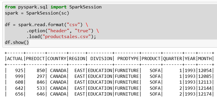
We have a few interesting columns in the sales data:

• Actual sales for the products by division
• Predicted sales for the products by division

If this were a bigger file, we could use SQL to determine the extent of the product list. Then the following is the Spark SQL to determine the product list:

df.groupBy("PRODUCT").count().show()  

The data frame groupBy function works very similar to the SQL Group By clause. Group By collects the items in the dataset according to the values in the column specified. In this case the PRODUCT column. The Group By results in a dataset being established with the results. As a dataset, we can query how many rows are in each with the count() function.

So, the result of the groupBy is a count of the number of items that correspond to the grouping element. For example, we grouped the items by CHAIR and found 288 of them:

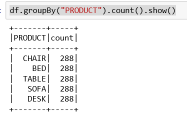
So, we obviously do not have real product data. It is unlikely that any company has the exact same number of products in each line.

We can look into the dataset to determine how the different divisions performed in actual versus predicted sales using the filter() command in this example:

df.filter(df['ACTUAL'] > df['PREDICT']).show()  

We pass a logical test to the filter command that will be operated against every row in the dataset. If the data in that row passes the test then the row is returned. Otherwise, the row is dropped from the results.

Our test is only interested in sales where the actual sales figure exceeds the predicted values.

Under Jupyter this looks as like the following:

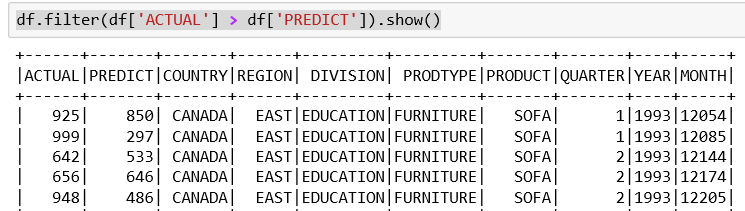
So, we get a reduced result set. Again, this was produced by the filter function as a data frame and can then be called upon to show as any other data frame. Notice the third record from the previous display is not present as its actual sales were less than predicted. It is always a good idea to use a quick survey to make sure you have the correct results.

What if we wanted to pursue this further and determine which were the best performing areas within the company?

If this were a database table we could create another column that stored the difference between actual and predicted sales and then sort our display on that column. We can perform very similar steps in Spark.

Using a data frame we could use coding like this:

#register dataframe as temporary SQL table
df.createOrReplaceTempView("sales")
# pull the values by the difference calculated
sqlDF = spark.sql("SELECT *, ACTUAL-PREDICT as DIFF FROM sales ORDER BY DIFF desc")
sqlDF.show()  

The first statement is creating a view/data frame within the context for further manipulation. This view is lazy evaluated, will not persist unless specific steps are taken, and most importantly can be accessed as a hive view. The view is available directly from the SparkContext.

We then create a new data frame with the computed new column using the new sales view that we created. Under Jupyter this looks as follows:

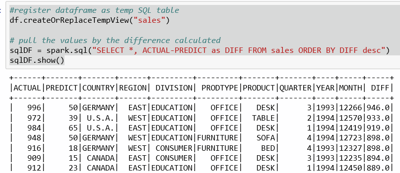
Again, I don't think we have realistic values as the differences are very far off from predicted values.