
Firstly, we will be creating the physical layer of our RPD.
The procedure is as follows:
- Start the Oracle BI Administration Tool by navigating to Programs | Oracle
BI | BI Administration. As shown in the following screenshot, in Oracle BI Administration Tool by clicking on File | New Repository...:

- This leads us to the start of the Create New Repository wizard. The first screen is an input screen for Repository Information where you need to input the following information:
- Name: Choose something sensible in this field according to the project or subject matter. For our purposes we will name the RPD as
AdventureWorks. - Location: Leave this field as it is, but this can be changed to anything that you require, such as a shared area or mapped drive.
- Repository Password: You must have at least eight characters and one numeral.
- Retype Password: Enter the same password that you entered in the Repository Password field.
- Import Metadata: If you choose Yes, you will automatically be prompted to import metadata (physical layer table definitions). If you choose No, a completely empty RPD will be created:

Go ahead and choose Yes. You will be presented with screens enabling you to automatically import physical table definitions, from a data source to the physical layer. We can create all of these definitions manually, using the Administration Tool, but a vast amount of time will be saved if the initial set of tables is imported with this method.
Within projects it is common to initially import a first draft of the schema directly from the database and then to make manual changes when needed as that schema is enhanced.
- Name: Choose something sensible in this field according to the project or subject matter. For our purposes we will name the RPD as
- In the first screen of the wizard, as shown in the following screenshot, you will need to choose the following:
- Connection Type: This can be a native driver for the major databases or via ODBC.
- Datasource Name: If we have chosen a native driver, for example Oracle, we will generally need to present this information.
- User Name: It is the user information for the data source.
- Password: It is needed for the Administration Tool so that it can access the data source. There are other bits of information that are required if you natively connect to other sources, for example, Essbase or Oracle OLAP. Have a play and choose other options from the Connection Type dropdown, and you will see those other requirements. For our purposes, we are using an SQL Server database and connecting to it via ODBC. This requires us to have SQL Server drivers installed on the local machine and a system DSN set up in the ODBC Data Source Administrator in Windows. These are quite common Windows/ODBC tasks, so we will not go into detail on setting this up. As you can see in the screenshot, we have an
AdventureworksDSN available that connects to our Data Warehouse schema. You have to input your User Name and Password. Then, click on Next: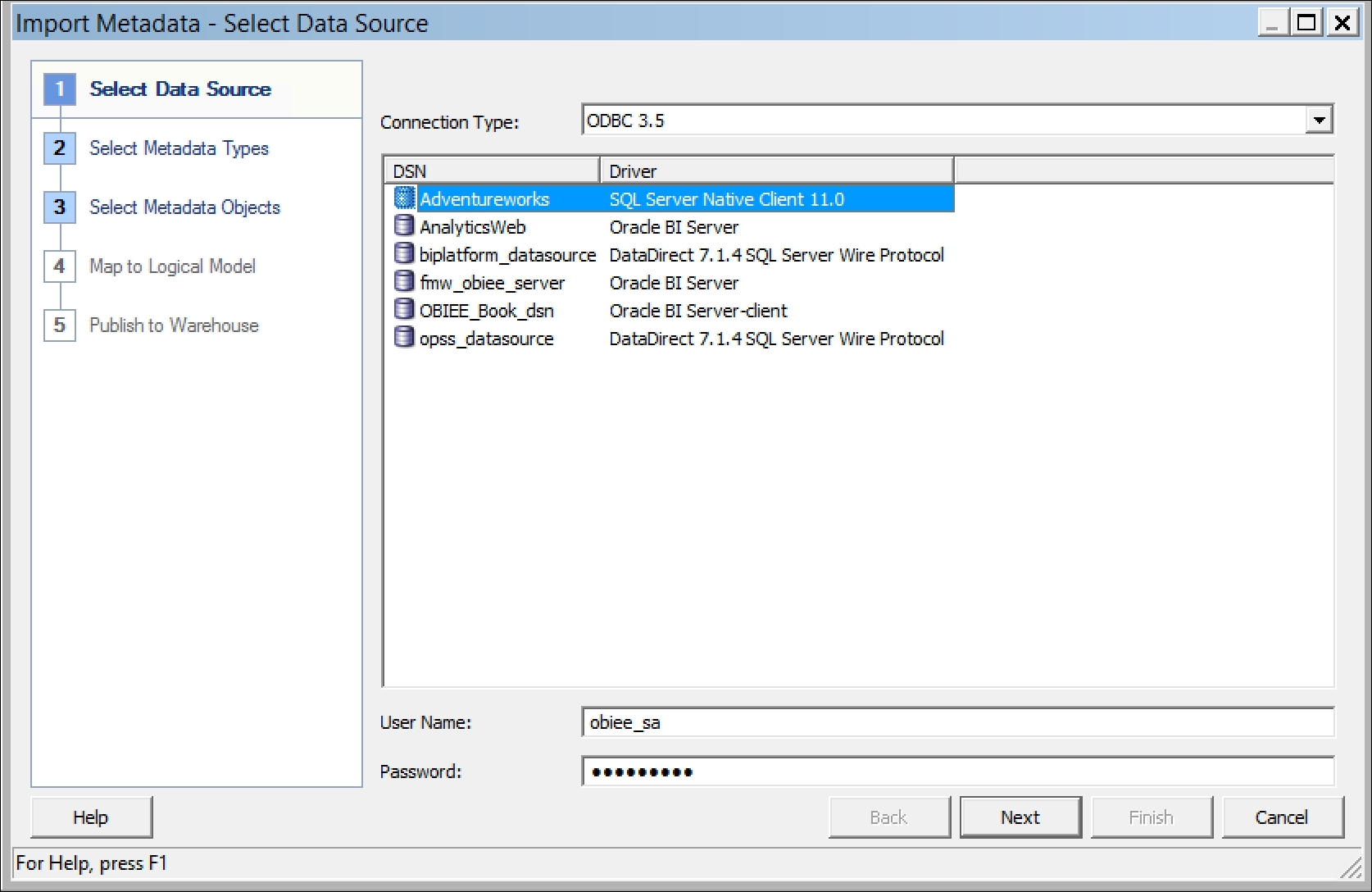
- In the following screen, choose which types of objects you want to import into the RPD. These are all common database terms that you should (hopefully!) be familiar with. For example, if you choose Views, in the next screen you will be able to import view definitions from the database. If you wish to import joins between tables, choose Keys and Foreign Keys:

The only non-generic option here is Metadata from CRM tables. If this is chosen, upon clicking the Nextbutton, the Administration Tool will read the table definitions in a legacy Siebel CRM system, from that CRM system's metadata dictionary. This is as opposed to reading these definitions directly from the database itself. Although this option is not widely used, it is important to note the distinction here. A CRM table may be different in definition at its application metadata layer compared to its implementation in the database, and project requirements may mean that the CRM application relationships are more pertinent.
We will ignore that CRM metadata. For our example, we have a very simple database schema, so we will only need to choose Tables, Keys, and Foreign Keys. Note that all foreign keys have not been set up in our database, so we will show you how to manually implement these in the Administration Tool as the chapter progresses.
- Once you are happy with our chosen options, click on Next. At this point, in the left-hand pane, you will see all the objects within the data source that we have provided details for, filtered by the options chosen in the previous screen:

If we were rerunning this wizard in the future, we may selectively choose objects and use the single arrow icon to move them to the right for importing. As we are starting from scratch, we will need all of these tables, so we can use the double arrow button to move everything into the right-hand pane. Once you do this, you can click on Finish and these table definitions will be imported.
- As shown in the following screenshot, at this point you will be in the main view of the RPD that you will see every time you return to open it. Note the structure, there you will see the base (physical) layer on the right-hand pane and the layers that build upon this flow to the left-hand side. Although initially this may be anti-intuitive to Western readers, this order does make sense when you consider how the metadata in the RPD actually works in a live environment. When building reports, we choose objects in the Presentationlayer. The tool then constructs an OBIEE-specific logical SQL that filters through the Business Model and Mapping layer. This, in turn, informs OBIEE how to turn that logical SQL into actual physical queries against our sources in the Physical layer.
These panes are, of course, empty at the moment, but we should see our imported tables in the Physical layer, waiting for us to check and finalize details such as the keys and joins.
Before we create joins, let's go through the Physical layer objects that have been automatically created by the Import Metadata wizard:

If you double-click on the topmost object, the Database object will open. This is more generically known as the Datasource, as we can have different types of source, for example, Flat files. Have a look at the following screenshot: in the General tab, we can set and amend features for that individual database connection. You can change the name of the object and if you decide to use another database type, we can inform OBIEE by changing that definition.
On this tab, there are also some useful advanced features, which we will briefly describe:
- Allow populate queries by default: This allows the use of this database to run and populate SQL.
- Allow direct database requests by default: This allows the execution of actual physical SQL queries directly against this database by passing the RPD metadata. Be extremely careful with this option, because if the connection rights within the connection pools (which we will discuss shortly) are too powerful, users will be able to do anything including dropping tables and updating data:

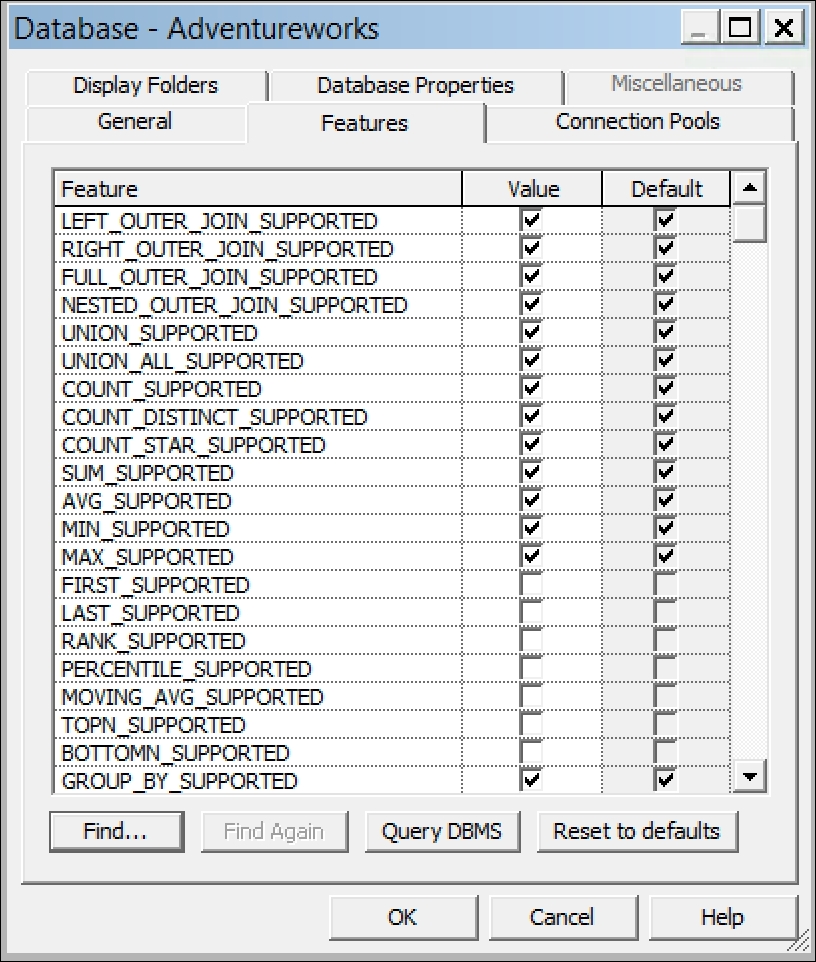
Moving onto the next tab--Features. Although this is an advanced part of the RPD, it is well worth quickly exploring this capability in the Database object. When we imported our table definitions, we stipulated the database type. The types of query that are supported by this specific database are populated, as shown in the following screenshot. You can then turn on or off supported types of query capability as you please. This results in the OBIEE server producing SQL that is restricted to the set of chosen features. This is sometimes really useful when fine-tuning queries against a certain database. However, be warned that this is an advanced feature and unless you are an experienced database developer or have DBA support, you should leave the default settings alone.
The next two tabs list the child objects of the database object, and we will cover these in the following sections.
Referring back to our physical layer, under the Database object we can see an item called Connection Pools. This contains authentication details for the database object and allows multiple users to use the same data source. We can also create multiple connection pools for the same data source. This may be helpful if you want to access the same data source, but with different users and their associated rights.
As shown in the following screenshot, in the General tab under Connection Pool, you can see the following fields:
- Name: It contains the name of the
Connection Poolobject. - Permissions: This button can be useful if you have multiple connection pools and want to restrict their use to certain groups of users. Be careful with this, as users will be able to access cached reports regardless of the permissions set here.
- Call interface: This field describes the method of connecting to the database object.
- Maximum connections: This determines the maximum number of connections that the server can open in the database through this connection pool. Before going live, take some time to get this setting right for your environment. You do not need to allow so many connections that query performance is degraded, or so few that users are frustrated as they cannot run queries. You will need to look at the capacity of your database to handle multiple concurrent sessions, and the size/memory of your servers. To get you started, we would say that it is useful to multiply the number of users on the system by the average number of queries on a dashboard.
Note
For example, a system has 100 users. Typically, 20 percent of them will be online, running an average of four reports at a time. So, our Maximum connections parameter will be as follows: (100 x 20 percent) x 4 = 80. Then, amend this number depending on our database capacity and as we assess how the system is used in a production environment.
- Timeout: Along with Maximum connections, this is an important setting as the time set here affects how often OBIEE opens and closes new connections. It is the field where we can stipulate how long a connection to a data source remains open. If a request is received within the set time, the associated query will use an open connection rather than creating a new one:

For our purposes, we are happy with the defaults that have been automatically created. Other advanced options are not relevant for our example project or most development activities, but it is worth having a look at the Connection Scripts tab (refer to the following screenshot). Here, it is possible to run commands on the database before and after the initiation of a query or database connection. This gives an opportunity to enhance the performance of requests against this connection pool. One example, from a recent project run by the authors of this book, is that we needed to improve the performance of a set of queries running against a specific connection pool. It was found to be really helpful to run the Alter Session command on the Oracle database to allow parallelism for SQL queries. Again, such a change would only be made after a very mature period of development and in consultation with your database experts:

Referring again to the objects that have been created automatically by the Import Metadata wizard, you can see an object called Adventureworks. This is called a Physical catalog. A catalog contains all of the definition information (metadata) for a particular data source (in our case, the database objects).
However, if we have vast amounts of metadata and want to organize objects that exist within the same schema in the database, we can optionally create a Physical Schema folder.
We have a small set of objects, so it is fine if we continue with the sole catalog, as the Import Metadata wizard has created.
Note
Physical Catalogs and Physical Schema (display) folders can be created by right-clicking on the data source. Additionally, Physical Schema folders can be created via the Display Folders tab within the Datasource object. A catalog contains information for a whole database object, while a schema contains metadata information for a schema owner. Model this in the same way that your database is designed.
Get your groups organized in advance. It is difficult to amend this afterwards, and if you decide to use folders instead of a catalog, you will not be able to rearrange and create a catalog.
Either of the previous objects will contain Physical tables. As we have mentioned in the preceding section, these are the definitions of the actual tables within our database. If you double-click on a Physical table object, you can see the basic properties of the table.
As with other objects, we can create physical table definitions manually by right-clicking on the catalog or schema folder. We can manipulate the definitions of columns and keys via their associated tabs or by expanding the physical table definitions and double-clicking on the individual columns.
We can also add foreign key relationships via the Foreign Keys tab. Let us take a look at the General, Columns, Keys, and Foreign Keys tabs in the following screenshots:


We can see that our column definitions have been imported correctly with a primary key (as denoted by the golden key sign). However, we do not seem to have any foreign keys. So, we will have to create these relationships (also known as physical joins) ourselves via the Administration Tool.
We could create the relationships between the tables by using the Foreign Keys tab, but the Administration Tool provides a far easier way of changing these relationships. This method uses what is called the Physical Diagram. During any development cycle, you will spend a lot of time in here. The Physical Diagram graphically represents relationships between tables. It will show basic cardinalities as with an Entity Relationship Diagram, that is, 1:M or 1:1 signifiers.
So, let's open the diagram. We can choose all of the tables that we want to model, then right-click on Physical Diagram | Selected Objects Only (actually, in this instance, any of those final options will suffice). Note that instead of a contextual right-click, we could have also used a button on the toolbar that looks like a mini-ERD diagram:

As you can see in the following screenshot, we are now presented with a graphical representation of the table definitions. We can double-click on the tables to open the previous screens that we discussed, but the most useful aspect of the diagram is that we can define the relationships between these tables in a visual manner:

To do this click on the New Join button (as denoted by the tooltip in the preceding screenshot) and then click on our fact table (FactFinance) and drag the pointer out to the table for which we want to define a join (in our case, theDimDate dimension).
As you can see in the screenshot, a line is drawn representing the relationship that exists between the two tables. The Physical Foreign Key screen prompts us. This is where we can stipulate the exact details of the join. OBIEE makes a pretty good guess of the join for single key tables, especially if we have already set up our primary keys properly.
In the following screenshot, we can see that it has guessed that we are joining on DateKey in both tables. This is correct, but if it had not been, we could easily change this in the Expression box. This would definitely need to be done if we were joining on compound keys. We would also have to check that the tables, columns, and join information are correct and have a look at the cardinality as well. Ensure that this is in line with your warehouse design: otherwise, redo the join:

Once you are happy with the settings, you can click on OK and proceed to define the joins for all other tables as needed. For each star within a warehouse, we will end up with something like what is shown in the following screenshot. The Physical Diagram is a great tool with which you can model your data. Visualizing your data in this way adds clarity and eases the development process:

Now we are ready to proceed to the next layer of the RPD. We have set up the objects needed for data connectivity and defined the objects that exist in that data source. Having completed a large amount of work, it is easy to make errors when completing large swathes of development. So we should save and check our work periodically. To this end, the Administration Tool provides what is commonly known as the consistency check, or in Oracle's own documentation as the Consistency Check Manager. This process will parse all of the metadata that we have developed, rather like one of the tasks a compiler may do for a programming language, and inform us of any errors. It will give us errors, which we must definitely fix before proceeding. Or it will create advisory warnings, where we can use our own judgment on whether it will impact our development negatively or not. Errors can range from missing object definitions, such as column types. Warnings can flag, as an example, a join that we have purposely disabled. We can also choose to have the process to give us best practice recommendations.
Normally, you will be prompted to run the check when saving your work, but it must be stressed that it is good practice to run this check of your own volition regularly. Let's run the check now. Select File | Check Global Consistency:

Ideally, next you should see the following message:
If not, and you see a list of errors and warnings, you will need to note this and look through your development to rectify these issues. There are too many possibilities to go through here, but as you increase in experience as an OBIEE developer, you will learn to recognize and solve these quickly.
Before we move onto the business layer, let's quickly look at a couple of best practices in developing this layer:
- Naming conventions: For ease of use, your objects should have identifiable names. For example, our physical tables have Dim and Fact prefixes denoting whether they are a dimension or fact. Another common standard is to have table name _D and _F suffixes.
- Aliases: If your physical objects are not appropriately named, you can create aliases by right-clicking on the object and choosing the alias creation option, as you can see in the following screenshot:

This creates another object, or level of abstraction, that retains its reference to the original source object. Then we can name this alias in a more appropriate way. Note that the icon for an alias differs:


Aliases are also commonly used to create multiple physical models based on the same base objects. This is sometimes useful if we want to avoid circular joins or just want to organize our Star schemas in a clear manner.