The business model is the highest level in this layer and it contains a business view of the physical schema. You should be able to simplify the physical schema so that in the end you get to look at the business view of the data. Anything we do in this layer will not affect the work that has been done in the physical layer, but we can create multiple models based on the same physical sources.To create a business model, right-click on the Business Model and Mapping pane in the middle and choose New Business Model. Then, we are prompted to give the model a name, as shown in the following screenshot:

We will name our model as AdventureWorkBM, and will keep the Disabled flag checked, as this model is not ready to handle any queries. Once we click on OK, we will see a new business model has been created. In the following screenshot, note that the business model icon is supplemented with a no entry sign. This signifies that it is disabled. We are now ready to start adding the logical representations of the tables that we have already added in the physical layer:

Within a business model, the most common object that you will create is called a logical table. This is a representation of one or more tables amalgamated into one logical group. A common best practice example would be if we have a Snowflake physical schema, we will be able to define that as a Star schema in the business model by combining multiple dimension tables as one logical dimension.

A logical table:

Initially, we are going to create a logical table for our Finance fact. Right-click on our new business model and select New Object | Logical Table:

Name the new table as Fact - Finance. We want this fact to contain measures from the FactFinance physical table. So, as shown in the following screenshot, we pick the required columns (in our case there is only one measure here, called Amount) in the physical layer and drag them to our new logical table:

Ideally, fact tables should only contain aggregated measures and dimension tables should only contain descriptive attributes.

As demonstrated in the following screenshot, after adding columns to that logical table, the Sources folder is now populated with a reference to the physical table that holds these columns. This is known as a logical table source:

A logical table source (LTS) is where you can map a logical table to one or more physical tables. As we will see later, we can use an LTS in the following ways:

We will cover these LTS scenarios as the chapter progresses, so let's concentrate on our current example. We have bought the measure over, but we need to tell the OBIEE server that these are metrics that should be shown in queries in an aggregated format defined by dimensions.

We will cover these LTS scenarios as the chapter progresses, so let's concentrate on our current example. We have bought the measure over, but we need to tell the OBIEE server that these are metrics that should be shown in queries in an aggregated format defined by dimensions. We do this by double-clicking on a column to get to the tabs shown in the following screenshot:

We will rename the column to something that makes more sense from a reporting point of view--Revenue. Note that this does not change the name of the physical column and that the mapping to that column will remain unaffected:

Then in the Aggregation tab, we will set the Default aggregation rule field to Sum, as this measure is an additive and we want to report on aggregated sales. Note that if we also want to treat this measure in a different manner, for example an average, we could copy this column and have the aggregation rule set to Avg. This would result in two logical columns, which are mapped to the same physical column, and will yield different results in a report due to our varying definitions in the business model:

Note that in the preceding screenshot, the name of the logical column has changed (without changing the underlying physical mapping). More importantly, the column is identified by a yellow slide rule icon, which indicates that this column has been defined as a measure.

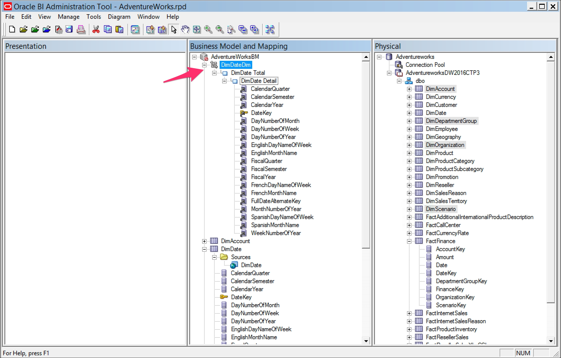
We will also go ahead and add a new logical table for a dimension. Rather than right- clicking, as we have done before, we can use the alternative method of dragging the whole physical table from the physical layer into the business model. Doing this for DimDate will result in what you can see in the following screenshot:

Note that when bringing the dimension table across, it also automatically sets one column (primary key) as a key for that logical table. Now, we do indeed need a logical key, but this should be something that has more of a business meaning. We can change this key in the same way that we did for a physical table: by opening the logical table, navigating to the Keys tab, and changing the key definition.

As with the joins in the physical layer, we must also set the relationships between logical tables. Again, the Administration Tool provides a good visual interface for this.

We can choose our dimension and fact. Right-click and select Business Model Diagram | Selected Tables and Direct Joins (as currently we only have two tables in the business layer, any option would have sufficed):

Refer to the way in which we set the joins between the tables in the physical layer. We can create joins in the business layer in exactly the same way. However, take a look at the join detail shown in the following screenshot. Notice that this time there are no columns stipulated in the Expression block for the join. This is because we previously already set up the physical relationships. The OBIEE server will use this information as well as the metadata that we have set up in the logical tables and logical table sources in order to ascertain what type of SQL query it should run:

Again, looking at the preceding information concerning a logical join, we do have a choice of what cardinality to set between these logical tables. This helps in providing the information to OBIEE on how to create queries. In general, you should leave this setting alone unless you are an advanced developer and understand the ramifications.

Now that we are comfortable with setting up logical facts and dimensions, let's go ahead and bring all of our Physical dimensions and facts into the business model:

Once we have done this, our RPD should look something like what you can see in the preceding screenshot. Note that we are using easily identifiable names for the logical tables. Also, we can see in the Business Model Diagram for this star, that all the tables are joined.

Now, there is a bit more work to do regarding dimensions. We need to create a dimension hierarchy for each logical dimension table.

At this point you may have been thinking about how to represent levels in a dimension. For example, how do we show that a geography dimension has levels of country, state, and city, or that time has year, month, and day? Well, OBIEE allows us to set hierarchies in the business model. The most common hierarchy is level-based. This enables us the following:

This results in the dimension object that you can see in the following screenshot. Notice that currently there are only two levels--one for the grand total and another for the lowest level of granularity. We need to have levels that correspond to a year, month, week, and so on. So there is a bit more work for us to do:

Build up the levels by starting at the lowest level and adding parents between that level and the grand total. We can do this by right-clicking and selecting New Object | Parent Level...:

As you can see in the following screenshot, we will be presented with the detail tabs. Our lowest level is Date, so we will name this next level up Week. Note that there is an entry called Number of Elements at this level. This entry does not affect the results that will be brought back in a query, but when we go on to include multiple table sources (especially aggregates), these figures will help the OBIEE server to optimize that query. Don't be worried about an exact number, all that matters are the ratios between levels. The grand total is defaulted to, and system set at 1. The lower levels should have numbers that are progressively higher.

In the example shown in the following screenshot, we are looking at the Week level. For our requirements, the next level will be Month. So, the final number that we input here will be just above four times of the number that we input at the Month level, as that is the ratio between a month and a week:

Remember that the ratio between levels matters more than the actual numbers.

If we do this for all of our new levels, we will end up with something resembling that is shown in the following screenshot. However, we also need to inform the OBIEE server about how to identify those levels using the columns that we have brought into the business layer. This requires us to set keys at each level:

Remember that we can also set drill paths within dimensions that can be utilized by the end users in their final reports. In addition to the level keys, it is at this point that we can set these keys:

So we need keys that uniquely identify a level, and we should not have columns at a level that differs from their grain. So, as an example, for our Time dimension, we have a very straightforward hierarchy of Year | Quarter | Month | Week | Date. We can see that we have unique identifiers such as MonthNumberOfYear for the month, WeekNumberOfYear for the week, and so on. These will be great for our level keys. Notice that we also have some descriptive columns, for example, EnglishMonthName. We need to ensure that these exist at the right level, so these will have to be moved as well. If we do that for all of the levels, we will get a hierarchy, as shown in the following screenshot:

At this point, we have still not stipulated which columns are keys and which are to be used in a drill path. We can do this by right-clicking on a column and choosing New Logical Level Key. We will then get a screen, as shown in the following screenshot. A Year, such as 2016, is both a unique identifier and a description that we would be happy to click on and drill down in a report. Therefore, we will set it as key, and check the Use for Display box to indicate that this is what we will be using for drilling in a report:

If we do this for all our levels, we will get a hierarchy, as shown in the following screenshot. Note that the icons have changed to a golden key, indicating that these are now keys. The keys that will uniquely identify these levels for optimization purposes are CalendarYear | CalendarQuarter | MonthNumberOfYear | WeekNumberofYear | DateKey. The drill path that we have set is CalendarYear | CalendarQuarter | EnglishMonthName | WeekNumberOfYear | EnglishDayNameOfWeek. Note that we have also removed superfluous columns, for example, French and Spanish Name columns:

Once we repeat this for all of our dimensions, we are ready for the final part of developing an RPD--the presentation layer.