A subject area is a grouping of objects from the business model. Note that, this can be a subset if required. We can do this by right-clicking in the presentation layer area and choosing the option to create a new subject area. We can then drag folders and columns across. We can also automatically create a subject area for the whole business model straight from the business layers. We do this by right-clicking in the Business Model and Mapping area and choosing Create Subject Areas for Logical Stars and Snowflakes:

This option automatically creates a separate subject area for each logical star that is detected. This can be a great way to start creating your subject areas.As you can see in the following screenshot, we have one subject area for our Finance star. Note that we have renamed that, and our AdventureWorks business model has a green 3D cube icon, which indicates that it has passed the consistency check and is now ready to generate queries. And also note that we have renamed our Time dimension hierarchy as Time Dim:

Also note the object in the presentation layer that is arrowed in the preceding screenshot. This is called a hierarchical column, and we will discuss this further in Chapter 8, Creating Dashboards and Analyses.

Development in this layer is not as involved as it is in others. It mostly involves considering how you wish to present your logical columns to the end user. End users will see tables and columns exactly as you arrange/name them in the presentation layer. Due to this flexibility, it's beneficial to go through some of the better practices that we have found through our own experience:

If you follow these guidelines with our example RPD, you will end up with something similar to what is shown in the following screenshot, in the Presentation layer: 

Note that we have removed the Dim prefixes and the columns have names with business meanings. We can reorder and rename tables by double-clicking on the subject area and navigating to the Presentation Tables tab, as shown in the following screenshot:

As you can see in the preceding screenshot, we can click on the pencil icon to rename a table. We can use the arrow buttons to reorder them.

We can make a subfolder by using a hyphen at the start of the presentation table name. This is especially useful as it is common to have an empty fact folder at the bottom with nested tables separating different types of measures.

Aliases

Have a look at the following screenshot:

We can see that there is also an Aliases tab. Here, we can rename a column without ever losing its mapping to a logical column. Every time we rename a column or table in the presentation layer, we retain a reference to the old presentation layer name here. This ensures that if we have already created reports and dashboards using these names, they will not create an error using the new names.

However, this also means that you cannot create a column/table with the old name unless that alias is deleted. This is a common source of errors, so be aware of this. Presentation aliases are easy to forget about, so you should use these very sparingly and keep in mind the drawbacks of using it. They should not be used as a quick way to fix badly named presentation objects. These have to be agreed with the business beforehand.

In the preceding screenshot, you can see the old name for the Finance subject area as an alias.

Many times users will try to choose columns from two or more dimensions in a report without choosing a fact. OBIEE will then choose a fact accordingly. However, this may not always be the fact that we desire the query path to run through. An example would be when you have multiple facts in one subject area that share conformed dimensions. Our current RPD doesn't have multiple facts. Let's say it did with shared Account and Scenario dimensions and we wanted to ensure that a query using those same two dimension always utilized the Finance fact. OBIEE allows for this by enabling the selection of an Implicit Fact for each subject area. We do this by double-clicking on a subject area and choosing Set for the Implicit Fact Column:

Then we choose any column from the fact that we want our default query to join to. So in the preceding example, you can see that we have opened the Finance subject area and are choosing a column from the Finance fact. Now, whenever we try to run a query in this subject area that consists solely of dimensions (that is, we don't specifically choose a measure from a fact table), this column and fact will be used for generating the query even if the OBIEE engine has a choice of multiple facts.

Note that this is not a mandatory step in development. An important part of a BI project involves educating end users. In general, properly educated users will not choose queries without a fact and they will have an awareness of their star structures. However, if you notice that this errant choice does commonly occur, think about implementing this feature.

Congratulations! We have finally completed the RPD. In albeit a simple example, we have gone through the process from start to finish. You can use this as a starting point in any environment. It's now time to delve into slightly more complicated examples of OBIEE functionality. As well as giving you greater insight into the full capability of OBIEE, it will also serve to reinforce concepts that we have already visited in this chapter.

So far, the columns and measures in our example RPD have had a one-to-one relationship with physical columns. We have added aggregation information, but we can also make new columns using already created logical columns and without the need to create new physical sources in the database.

For this example, we will use the InternetSales fact. We won't step through the modeling from the physical layer to the presentation layer as the methods are exactly as for the Finance fact that we have already completed. Please refer to the sample AdventureWorks RPD if you need to reference.

In this fact, we have measures for Sales Amount and Total Product Cost, but let's say that we have a requirement to understand what the profit margin is on a product. To do this, right-click on our logical table and choose New Object | Logical Column...:

Then you will get the screen shown in the following screenshot. In the General tab, name our new measure as Gross Product Profit. Then proceed to the Column Source tab. Note that there is no physical column currently mapped. Remember from the preceding section that we dragged objects from the physical layer to the business layer, automatically creating logical columns with their appropriate physical mapping:

This time, we are creating a column directly in the business layer. We are not worried about physical mappings or columns as we can deduce the information for the new measure from two current logical columns. So, as you can see in the preceding screenshot, we have checked the Derived from existing columns using an expression option. If you are familiar with the syntax needed, you can type that into the input box straightaway. Alternatively, you can invoke the Expression Builder by clicking on the icon with the fx indicator on the bottom right of the screen, shown in the preceding screenshot.

You will come across the Expression Builder in many places during project development. It exposes functions and methods of manipulating data that the OBIEE server provides. We can use these to create new definitions in a repository. One function enables us to manipulate strings in an attribute column, for example, concatenating the first name and last name for a customer. Another function allows us to convert a column data type. In fact, there are many possibilities here, and you are well advised to take the time to explore the functionality available here. You can have a look at the various functions and objects by changing the choice in the Category box in the top left of the screen shown in the following screenshot. Then you will be given further options in the other two boxes:

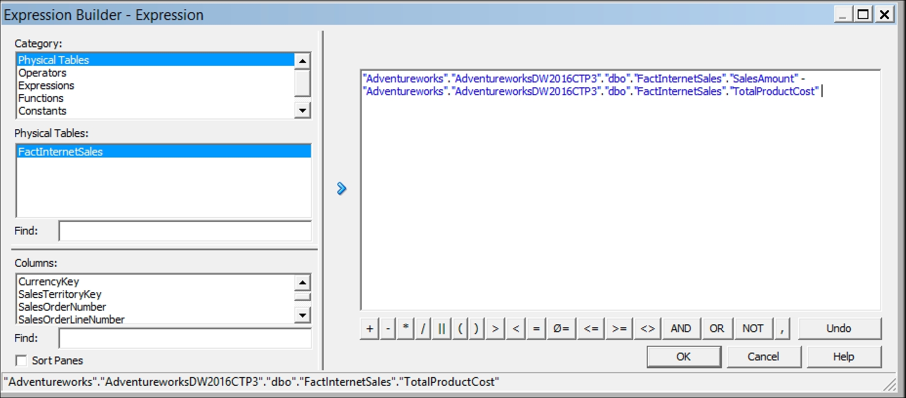
In our case, we want to refer to two logical columns. So choose Logical Tables as our Category and then choose the table (Fact - InternetSales) and columns that we require. We can then make a calculation that represents the profit margin. You can see that calculation in the preceding screenshot.

Once you click on OK, the Expression Builder will check that our syntax is coherent and if it parses successfully then you can proceed to drag this new measure to our physical layer. Note that in the Column Source tab, the column automatically gets a data type of INT and the Aggregation tab is grayed out. Both of these are derived from our base columns.

So now we have a new measure that our business can use without having to alter our original physical data source. All the required development has taken place within OBIEE:

We can create the same calculation, but this time using physical columns rather than logical columns as our base. So we will create a new logical column exactly as before; however, let's name it as Gross Product Profit (Physical). Note that this time we have to set an aggregation rule as we are deriving the information straight from physical columns instead of logical ones. After this, we need to open the logical table source. We can do this via the Column Source tab and edit the logical source from the Derived from physical mappings section (previously we used the Expression Builder), or we can double-click on the LTS (Logical Table Source) itself. Then we proceed to the Column Mapping tab, as you can see in the following screenshot:

In the preceding screenshot, you can see the mappings from physical to logical columns. If you check the Show unmapped columns box, you will see our new logical column. To create the mapping and calculation, choose our new column and again click on the Expression Builder icon:

This time we do not have access to logical columns and tables. They have been replaced by physical tables, but we have access to the same functions and operators. If our syntax is correct, we can drag this column to the presentation layer.

Although we have discussed two separate methods to produce the exact same calculation, you have to be careful when choosing the solution for a live environment. The rather more correct method in this case would be to use a physical calculation. Why? Well, because we want to know the aggregated profit margin and then aggregate upwards. So, it is better that we set an aggregation rule after our calculation, rather than setting it before, as it is in the first case. If we had another example, for example, finding a percentage between two already aggregated amounts, then the logical calculation would be better as we are aggregating before the final calculation:

However, the best advice, as always, is to test your results and experiment freely as you learn so that your knowledge of the system, its capabilities, and its limitations increases. Both of these methods will be utilized as needed according to your project requirements. Ensure that you test the results properly before you expose such development to the users.

OBIEE also provides several functions that allow you to make comparisons between different time periods. For example, we may have a report based on the current month's sales, but we also want to include a column for last month's sales as well so that we can compare. OBIEE offers the following time series functions:

We do this by double-clicking on the Time dimension hierarchy in the business layer and ensuring that the Time box is checked under the Structure options. This will then give us the option to set a chronological key at each level of the dimension, as shown in the following screenshot:

The OBIEE server requires a chronological key to be set for each level of our Time hierarchy. Oracle describes this key as monotonically increasing, which for our purposes means a key that increases in chronological order. This key will enable the server to produce efficient SQL when creating the time series queries:

As you can see in the preceding screenshot, we have opened the detail level of our hierarchy and set the key. Then proceed to do the same for all of our levels. At this point, we are ready to create our new measure.

First, create a new logical measure in the business layer. We will be doing this in our Fact - Finance logical fact table. As we showed you in the preceding section, we will open the Expression Builder to create our calculation from an already existing logical column. If we choose AGO from the time series function, the builder will ask us to create a calculation based on this syntax:

Ago(<<Measure>>,<<Level>>,<<Number of Periods>>)

The measure we want to make a comparison with is Revenue, and let's say our requirement is to see the previous year's sales. Choose the Year level from our Time dimension (as you can see in the following screenshot). The number of periods will be 1 as we wish to have a time-shift of one year:

Drag this measure to the presentation layer, and there you go, we have a new measure based on the AGO function. We now can show current revenue and last year's revenue for the same chosen dimensions in the same report. Note that we could have built this measure upon a column that was calculated from two other logical columns, for example, from our InternetSales fact as previously shown. This shows how you can increase complexity in the business layer without changing physical columns, and how quickly you can increase the sophistication of your offering to the end users.

Now you may remember that we set the Number of elements at this level for each logical level. That helps the server with general queries. You can also help the server specifically optimize time series functions by adding Sequence Numbers for each logical level. This is new to 12c and can be done via the Sequence Numbers tab. You have two choices of sequencing that you can input:

The AGO measure will show us last year's results for the lowest grain in our report. So if we were looking for a report by month, that measure would show us the data for the same month last year. How about if we wanted to show data for the whole previous year, in spite of the grain that we choose for our report? Well, we can leverage our dimensional hierarchy and create a measure that always covers an entire year. This is done by creating a measure and setting its content level to the desired level in one of our dimensions.

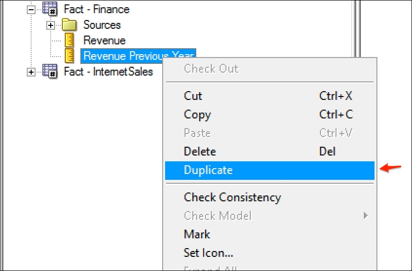
Again, we will build upon our previous work. As you can see in the following screenshot, you can copy the whole definition of our AGO measure by right-clicking and choosing Duplicate:

Then open this new logical column, rename it, and navigate to the Levels tab. The Levels tab shows us all of the levels for the dimensions that we have connected to this logical table:

In our case, as you can see in the preceding screenshot, choose the Year level from the Time dimension. This means that this measure will always show results for an aggregated level of Year. This functionality is extremely useful when dealing with many requirements. For example, a business may need to compare the sales performance of a store against that of its parent region, but they are in different levels in the same dimension. We could create a level-based measure for the parent region and still show results for the store.

Once you have clicked on OK, our new measure is created:

As shown in the preceding screenshot, this new measure now appears in our dimension hierarchy for Time and at the Year level. This shows that this column/measure is always aggregated at this level of the Time dimension. Note that rather than changing the settings in the Levels tab, we could also have dragged this new measure to the Year level in the hierarchy. Both methods yield the same end result.