
Recurrent neural networks are really good at analyzing sequential and time-series data. You can learn more about them at http://www.wildml.com/2015/09/recurrent-neural-networks-tutorial-part-1-introduction-to-rnns. When we deal with sequential and time-series data, we cannot just extend generic models. The temporal dependencies in the data are really important, and we need to account for this in our models. Let's look at how to build them.
- Create a new Python file, and import the following packages:
import numpy as np
import matplotlib.pyplot as plt
import neurolab as nl
- Define a function to create a waveform, based on input parameters:
def create_waveform(num_points): # Create train samples data1 = 1 * np.cos(np.arange(0, num_points)) data2 = 2 * np.cos(np.arange(0, num_points)) data3 = 3 * np.cos(np.arange(0, num_points)) data4 = 4 * np.cos(np.arange(0, num_points)) - Create different amplitudes for each interval to create a random waveform:
# Create varying amplitudes amp1 = np.ones(num_points) amp2 = 4 + np.zeros(num_points) amp3 = 2 * np.ones(num_points) amp4 = 0.5 + np.zeros(num_points) - Combine the arrays to create the output arrays. This data corresponds to the input and the amplitude corresponds to the labels:
data = np.array([data1, data2, data3, data4]).reshape(num_points * 4, 1) amplitude = np.array([[amp1, amp2, amp3, amp4]]).reshape(num_points * 4, 1) return data, amplitude - Define a function to draw the output after passing the data through the trained neural network:
# Draw the output using the network def draw_output(net, num_points_test): data_test, amplitude_test = create_waveform(num_points_test) output_test = net.sim(data_test) plt.plot(amplitude_test.reshape(num_points_test * 4)) plt.plot(output_test.reshape(num_points_test * 4)) - Define the
mainfunction and start by creating sample data:if __name__=='__main__': # Get data num_points = 30 data, amplitude = create_waveform(num_points) - Create a recurrent neural network with two layers:
# Create network with 2 layers net = nl.net.newelm([[-2, 2]], [10, 1], [nl.trans.TanSig(), nl.trans.PureLin()]) - Set the initialized functions for each layer:
# Set initialized functions and init net.layers[0].initf = nl.init.InitRand([-0.1, 0.1], 'wb') net.layers[1].initf= nl.init.InitRand([-0.1, 0.1], 'wb') net.init() - Train the recurrent neural network:
# Training the recurrent neural network error = net.train(data, amplitude, epochs=1000, show=100, goal=0.01) - Compute the output from the network for the training data:
# Compute output from network output = net.sim(data) - Plot training error:
# Plot training results plt.subplot(211) plt.plot(error) plt.xlabel('Number of epochs') plt.ylabel('Error (MSE)') - Plot the results:
plt.subplot(212) plt.plot(amplitude.reshape(num_points * 4)) plt.plot(output.reshape(num_points * 4)) plt.legend(['Ground truth', 'Predicted output']) - Create a waveform of random length and see whether the network can predict it:
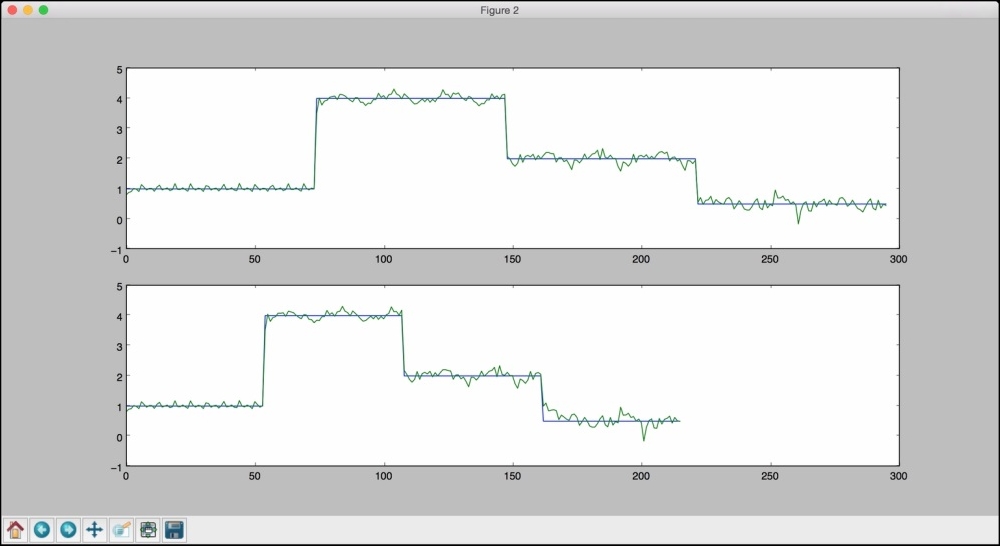
# Testing on unknown data at multiple scales plt.figure() plt.subplot(211) draw_output(net, 74) plt.xlim([0, 300]) - Create another waveform of a shorter length and see whether the network can predict it:
plt.subplot(212) draw_output(net, 54) plt.xlim([0, 300]) plt.show() - The full code is in the
recurrent_network.pyfile that's already provided to you. If you run this code, you will see two figures. The first figure displays training errors and the performance on the training data: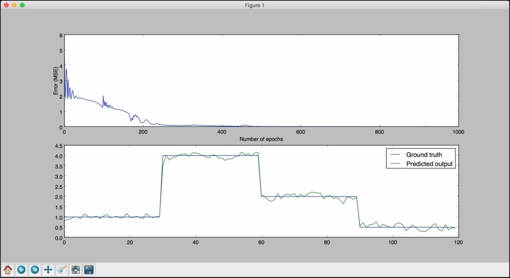
The second figure displays how a trained recurrent neural net performs on sequences of arbitrary lengths:
You will see the following on your Terminal:
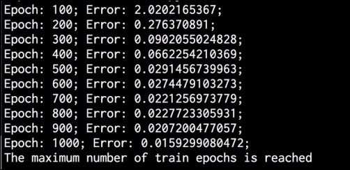
..................Content has been hidden....................
You can't read the all page of ebook, please click here login for view all page.