
In the preceding chapter, we looked at some widely-used dimensionality reduction techniques, which enable a data scientist to get greater insight into the nature of datasets.
The next few chapters will focus on some more sophisticated techniques, drawing from the area of deep learning. This chapter is dedicated to building an understanding of how to apply the Restricted Boltzmann Machine (RBM) and manage the deep learning architecture one can create by chaining RBMs—the deep belief network (DBN). DBNs are trainable to effectively solve complex problems in text, image, and sound recognition. They are used by leading companies for object recognition, intelligent image search, and robotic spatial recognition.
The first thing that we're going to do is get a solid grounding in the algorithm underlying DBN; unlike clustering or PCA, this code isn't widely-known by data scientists and we're going to review it in some depth to build a strong working knowledge. Once we've worked through the theory, we'll build upon it by stepping through code that brings the theory into focus and allows us to apply the technique to real-world data. The diagnosis of these techniques is not trivial and needs to be rigorous, so we'll emphasize the thought processes and diagnostic techniques that enable us to effectively watch and control the success of your implementation.
By the end of this chapter, you'll understand how the RBM and DBN algorithms work, know how to use them, and feel confident in your ability to improve the quality of the results you get out of them. To summarize, the contents of this chapter are as follows:
- Neural networks – a primer
- Restricted Boltzmann Machines
- Deep belief networks
The RBM is a form of recurrent neural network. In order to understand how the RBM works, it is necessary to have a more general understanding of neural networks. Readers with an understanding of artificial neural network (hereafter neural network, for the sake of simplicity) algorithms will find familiar elements in the following description.
There are many accounts that cover neural networks in great theoretical detail; we won't go into great detail retreading this ground. For the purposes of this chapter, we will first describe the components of a neural network, common architectures, and prevalent learning processes.
For unfamiliar readers, neural networks are a class of mathematical models that train to produce and optimize a definition for a function (or distribution) over a set of input features. The specific objective of a given neural network application can be defined by the operator using a performance measure (typically a cost function); in this way, neural networks may be used to classify, predict, or transform their inputs.
The use of the word neural in neural networks is the product of a long tradition of drawing from heavy-handed biological metaphors to inspire machine learning research. Hence, artificial neural networks algorithms originally drew (and frequently still draw) from biological neuronal structures.
A neural network is composed of the following elements:
- A learning process: A neural network learns by adjusting parameters within the weight function of its nodes. This occurs by feeding the output of a performance measure (as described previously, in supervised learning contexts this is frequently a cost function, some measure of inaccuracy relative to the target output of the network) into the learning function of the network. This learning function outputs the required weight adjustments (Technically, it typically calculates the partial derivatives—terms required by gradient descent.) to minimize the cost function.
- A set of neurons or weights: Each contains a weight function (the activation function) that manipulates input data. The activation function may vary substantially between networks (with one well-known example being the hyperbolic tangent). The key requirement is that the weights must be adaptive, that is,, adjustable based on updates from the learning process. In order to model non-parametrically (that is, to model effectively without defining details of the probability distribution), it is necessary to use both visible and hidden units. Hidden units are never observed.
- Connectivity functions: They control which nodes can relay data to which other nodes. Nodes may be able to freely relay input to one another in an unrestricted or restricted fashion, or they may be more structured in layers through which input data must flow in a directed fashion. There is a broad range of interconnection patterns, with different patterns producing very different network properties and possibilities.
Utilizing this set of elements enables us to build a broad range of neural networks, ranging from the familiar directed acyclic graph (with perhaps the best-known example being the Multi-Layer Perceptron (MLP)) to creative alternatives. The Self-Organizing Map (SOM) that we employed in the preceding chapter was a type of neural network, with a unique learning process. The algorithm that we'll examine later in this chapter, that of the RBM, is another neural network algorithm with some unique properties.
There are many variations on how the neurons in a neural network are connected, with structural decisions being an important factor in determining the network's learning capabilities. Common topologies in unsupervised learning tend to differ from those common to supervised learning. One common and now familiar unsupervised learning topology is that of the SOM that we discussed in the last chapter.
The SOM, as we saw, directly projects individual input cases onto a weight vector contained by each node. It then proceeds to reorder these nodes until an appropriate mapping of the dataset is converged on. The actual structure of the SOM was a variant based on the details of training, specific outcome of a given instance of training, and design decisions taken in structuring the network, but square or hexagonal grid structures are becoming increasingly common.
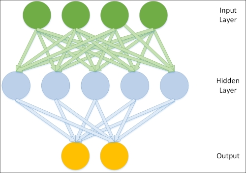
A very common topology type in supervised learning is that of a three-layer, feedforward network, with the classical case being the MLP. In this network topology model, the neurons in the network are split into layers, with each layer communicating to the layer "beyond" it. The first layer contains inputs that are fed to a hidden layer. The hidden layer develops a representation of the data using weight activations (with the right activation function, for example, sigmoid or gauss, an MLP can act as a universal function approximator) and activation values are communicated to the output layer. The output layer typically delivers network results. This topology, therefore, looks as follows:
Other network topologies deliver different capabilities. The topology of a Boltzmann Machine, for instance, differs from those described previously. The Boltzmann machine contains hidden and visible neurons, like those of a three-layer network, but all of these neurons are connected to one another in a directed, cyclic graph:
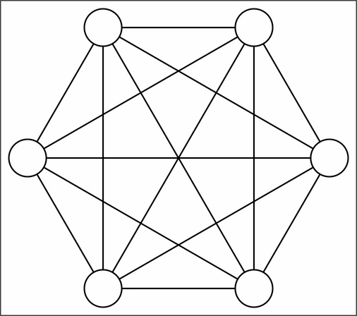
This topology makes Boltzmann machines stochastic—probabilistic rather than deterministic—and able to develop in one of several ways given a sufficiently complex problem. The Boltzmann machine is also generative, which means that it is able to fully (probabilistically) model all of the input variables, rather than using the observed variables to specifically model the target variables.
Which network topology is appropriate depends to a large extent on your specific challenge and the desired output. Each tends to be strong in certain areas. Furthermore, each of the topologies described here will be accompanied by a learning process that enables the network to iteratively converge on an (ideally optimal) solution.
There are a broad range of learning processes, with specific processes and topologies being more or less compatible with one another. The purpose of a learning process is to enable the network to adjust its weights, iteratively, in such a way as to create an increasingly accurate representation of the input data.
As with network topologies, there are a great many learning processes to consider. Some familiarity is assumed and a great many excellent resources on learning processes exist (some good examples are given at the end of this chapter). This section will focus on delivering a common characterization of learning processes, while later in the chapter, we'll look in greater detail at a specific example.
As noted, the objective of learning in a neural network is to iteratively improve the distribution of weights across the model so that it approximates the function underlying input data with increasing accuracy. This process requires a performance measure. This may be a classification error measure, as is commonly used in supervised, classification contexts (that is, with the backpropagation learning algorithm in MLP networks). In stochastic networks, it may be a probability maximization term (such as energy in energy-based networks).
In either case, once there is a measure to increase probability, the network is effectively attempting to reduce that measure using an optimization method. In many cases, the optimization of the network is achieved using gradient descent. As far as the gradient descent algorithm method is concerned, the size of your performance measure value on a given training iteration is analogous to the slope of your gradient. Minimizing the performance measure is therefore a question of descending that gradient to the point at which the error measure is at its lowest for that set of weights.
The size of the network's updates for the next iteration (the learning rate of your algorithm) may be influenced by the magnitude of your performance measure, or it may be hard-coded.
The weight updates by which your network adjusts may be derived from the error surface itself; if so, your network will typically have a means of calculating the gradient, that is, deriving the values to which updates need to adjust the parameters on your network's activated weight functions so as to continue to reduce the performance measure.
Having reviewed the general concepts underlying network topologies and learning methods, let's move into the discussion of a specific neural network, the RBM. As we'll see, the RBM is a key part of a powerful deep learning algorithm.