
We've discussed what semi-supervised learning is, why we want to engage in it, and what some of the general realities of employing semi-supervised algorithms are. We've gone about as far as we can with general descriptions. Over the next few pages, we'll move from this general understanding to develop an ability to use a semi-supervised application effectively.
Self-training is the simplest semi-supervised learning method and can also be the fastest. Self-training algorithms see an application in multiple contexts, including NLP and computer vision; as we'll see, they can present both substantial value and significant risks.
The objective of self-training is to combine information from unlabeled cases with that of labeled cases to iteratively identify labels for the dataset's unlabeled examples. On each iteration, the labeled training set is enlarged until the entire dataset is labeled.
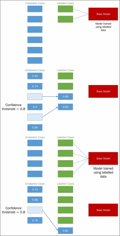
The self-training algorithm is typically applied as a wrapper to a base model. In this chapter, we'll be using an SVM as the base for our self-training model. The self-training algorithm is quite simple and contains very few steps, as follows:
- A set of labeled data is used to predict labels for a set of unlabeled data. (This may be all unlabeled data or part of it.)
- Confidence is calculated for all newly labeled cases.
- Cases are selected from the newly labeled data to be kept for the next iteration.
- The model trains on all labeled cases, including cases selected in previous iterations.
- The model iterates through steps 1 to 4 until it successfully converges.
Presented graphically, this process looks as follows:
Upon completing training, the self-trained model would be tested and validated. This may be done via cross-validation or even using held-out, labeled data, should this exist.
Self-training provides real power and time saving, but is also a risky process. In order to understand what to look out for and how to apply self-training to your own classification algorithms, let's look in more detail at how the algorithm works.
To support this discussion, we're going to work with code from the semisup-learn GitHub repository. In order to use this code, we'll need to clone the relevant GitHub repository. Instructions for this are located in Appendix A.
The first step in each iteration of self-training is one in which class labels are generated for unlabeled cases. This is achieved by first creating a SelfLearningModel class, which takes a base supervised model (basemodel) and an iteration limit as arguments. As we'll see later in this chapter, an iteration limit can be explicitly specified or provided as a function of classification accuracy (that is, convergence). The prob_threshold parameter provides a minimum quality bar for label acceptance; any projected label that scores at less than this level will be rejected. Again, we'll see in later examples that there are alternatives to providing a hardcoded threshold value.
class SelfLearningModel(BaseEstimator):


def __init__(self, basemodel, max_iter = 200, prob_threshold = 0.8):
   self.model = basemodel
   self.max_iter = max_iter
   self.prob_threshold = prob_threshold
Having defined the shell of the SelfLearningModel class, the next step is to define functions for the process of semi-supervised model fitting:
def fit(self, X, y):
   unlabeledX = X[y==-1, :]
   labeledX = X[y!=-1, :]
   labeledy = y[y!=-1]

   self.model.fit(labeledX, labeledy)
   unlabeledy = self.predict(unlabeledX)
   unlabeledprob = self.predict_proba(unlabeledX)
   unlabeledy_old = []

   i = 0
The X parameter is a matrix of input data, whose shape is equivalent to [n_samples, n_features]. X is used to create a matrix of [n_samples, n_samples] size. The y parameter, meanwhile, is an array of labels. Unlabeled points are marked as -1 in y. From X, the unlabeledX and labeledX parameters are created quite simply by operations over X that select elements in X whose position corresponds to a -1 label in y. The labeledy parameter performs a similar selection over y. (Naturally, we're not that interested in the unlabeled samples of y as a variable, but we need the labels that do exist for classification attempts!)
The actual process of label prediction is achieved, first, using sklearn's predict operation. The unlabeledy parameter is generated using sklearn's predict method, while the predict_proba method is used to calculate probabilities for each projected label. These probabilities are stored in unlabeledprob.
Note
Scikit-learn's predict and predict_proba methods work to predict class labels and the probability of class labeling being correct, respectively. As we'll be applying both of these methods within several of our semi-supervised algorithms, it's informative to understand how they actually work.
The predict method produces class predictions for input data. It does so via a set of binary classifiers (that is, classifiers that attempt to differentiate only two classes). A full model with n-many classes contains a set of binary classifiers as follows:

In order to make a prediction for a given case, all classifiers whose scores exceed zero, vote for a class label to apply to that case. The class with the most votes (and not, say, the highest sum classifier score) is identified. This is referred to as a one-versus-one prediction method and is a fairly common approach.
Meanwhile, predict_proba works by invoking
Platt calibration, a technique that allows the outputs of a classification model to be transformed into a probability distribution over the classes. This involves first training the base model in question, fitting a regression model to the classifier's scores:
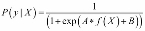
This model can then be optimized (through scalar parameters A and B) using a maximum likelihood method. In the case of our self-training model, predict_proba allows us to fit a regression model to the classifier's scores and thus calculate probabilities for each class label. This is extremely helpful!
Next, we need a loop for iteration. The following code describes a while loop that executes until there are no cases left in unlabeledy_old (a copy of unlabeledy) or until the max iteration count is reached. On each iteration, a labeling attempt is made for each case that does not have a label whose probability exceeds the probability threshold (prob_threshold):
   while (len(unlabeledy_old) == 0 or
      numpy.any(unlabeledy!=unlabeledy_old)) and i < self.max_iter:
      unlabeledy_old = numpy.copy(unlabeledy)
      uidx = numpy.where((unlabeledprob[:, 0] > self.prob_threshold)
      | (unlabeledprob[:, 1] > self.prob_threshold))[0]
The self.model.fit method then attempts to fit a model to the unlabeled data. This unlabeled data is presented in a matrix of size [n_samples, n_samples] (as referred to earlier in this chapter). This matrix is created by appending (with vstack and hstack) the unlabeled cases:
      self.model.fit(numpy.vstack((labeledX, unlabeledX[uidx, :])),
      numpy.hstack((labeledy, unlabeledy_old[uidx])))
Finally, the iteration performs label predictions, followed by probability predictions for those labels.
      unlabeledy = self.predict(unlabeledX)
      unlabeledprob = self.predict_proba(unlabeledX)
      i += 1
On the next iteration, the model will perform the same process, this time taking the newly labeled data whose probability predictions exceeded the threshold as part of the dataset used in the model.fit step.
If one's model does not already include a classification method that can generate label predictions (like the predict_proba method available in sklearn's SVM implementation), it is possible to introduce one. The following code checks for the predict_proba method and introduces Platt scaling of generated labels if this method is not found:
if not getattr(self.model, "predict_proba", None):
   self.plattlr = LR()
   preds = self.model.predict(labeledX)
   self.plattlr.fit( preds.reshape( -1, 1 ), labeledy )

return self


def predict_proba(self, X):
         if getattr(self.model, "predict_proba", None):
         return self.model.predict_proba(X)
         else:
            preds = self.model.predict(X)
            return self.plattlr.predict_proba(preds.reshape( -1, 1 ))
Once we have this much in place, we can begin applying our self-training architecture. To do so, let's grab a dataset and start working!
For this example, we'll use a simple linear regression classifier, with Stochastic Gradient Descent (SGD) as our learning component as our base model (basemodel). The input dataset will be the statlog
heart dataset, obtained from www.mldata.org. This dataset is provided in the GitHub repository accompanying this chapter.
The heart dataset is a two-class dataset, where the classes are the absence or presence of a heart disease. There are no missing values across the 270 cases for any of its 13 features. This data is unlabeled and many of the variables needed are usually captured via expensive and sometimes inconvenient tests. The variables are as follows:
agesexchest pain type (4 values)resting blood pressureserum cholestoral in mg/dlfasting blood sugar > 120 mg/dlresting electrocardiographic results (values 0,1,2)maximum heart rate achievedexercise induced angina10. oldpeak = ST depression induced by exercise relative to restthe slope of the peak exercise ST segmentnumber of major vessels (0-3) colored by flourosopythal: 3 = normal; 6 = fixed defect; 7 = reversable defect
Lets get started with the Heart dataset by loading in the data, then fitting a model to it:
heart = fetch_mldata("heart")
X = heart.data
ytrue = np.copy(heart.target)
ytrue[ytrue==-1]=0

labeled_N = 2
ys = np.array([-1]*len(ytrue)) # -1 denotes unlabeled point
random_labeled_points = random.sample(np.where(ytrue == 0)[0], labeled_N/2)+
andom.sample(np.where(ytrue == 1)[0], labeled_N/2)
ys[random_labeled_points] = ytrue[random_labeled_points]

basemodel = SGDClassifier(loss='log', penalty='l1')

basemodel.fit(X[random_labeled_points, :], ys[random_labeled_points])
print "supervised log.reg. score", basemodel.score(X, ytrue)

ssmodel = SelfLearningModel(basemodel)
ssmodel.fit(X, ys)
print "self-learning log.reg. score", ssmodel.score(X, ytrue)
Attempting this yields moderate, but not excellent, results:
self-learning log.reg. score 0.470347
However, over 1,000 trials, we find that the quality of our outputs is quite variant:
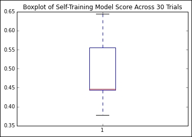
Given that we're looking at classification accuracy scores for sets of real-world and unlabeled data, this isn't a terrible result, but I don't think we should be satisfied with it. We're still labeling more than half of our cases incorrectly!
We need to understand the problem a little better; right now, it isn't clear what's going wrong or how we can improve on our results. Let's figure this out by returning to the theory around self-training to understand how we can diagnose and improve our implementation.
In the previous section, we discussed the creation of self-training algorithms and tried out an implementation. However, what we saw during our first trial was that our results, while demonstrating the potential of self-training, left room for growth. Both the accuracy and variance of our results were questionable.
Self-training can be a fragile process. If an element of the algorithm is ill-configured or the input data contains peculiarities, it is very likely that the iterative process will fail once and continue to compound that error by reintroducing incorrectly labeled data to future labeling steps. As the self-training algorithm iteratively feeds itself, garbage in, garbage out is a very real concern.
There are several quite common flavors of risk that should be called out. In some cases, labeled data may not add more useful information. This is particularly common in the first few iterations, and understandably so! In general, unlabeled cases that are most easily labeled are the ones that are most similar to existing labeled cases. However, while it's easy to generate high-probability labels for these cases, there's no guarantee that their addition to the labeled set will make it easier to label during subsequent iterations.
Unfortunately, this can sometimes lead to a situation in which cases are being added that have no real effect on classification while classification accuracy in general deteriorates. Even worse, adding cases that are similar to pre-existing cases in enough respects to make them easy to label, but that actually misguide the classifier's decision boundary, can introduce misclassification increases.
Diagnosing what went wrong with a self-training model can sometimes be difficult, but as always, a few well-chosen plots add a lot of clarity to the situation. As this type of error occurs particularly often within the first few iterations, simply adding an element to the label prediction loop that writes the current classification accuracy allows us to understand how accuracy trended during early iterations.
Once the issue has been identified, there are a few possible solutions. If enough labeled data exists, a simple solution is to attempt to use a more diverse set of labeled data to kick-start the process.
While the impulse might be to use all of the labeled data, we'll see later in this chapter that self-training models are vulnerable to overfitting—a risk that forces us to hold on to some data for validation purposes. A promising option is to use multiple subsets of our dataset to train multiple self-training model instances. Doing so, particularly over several trials, can help us understand the impact of our input data on our self-training models performance.
In Chapter 8, Ensemble Methods, we'll explore some options around ensembles that will enable us to use multiple self-training models together to yield predictions. When ensembling is accessible to us, we can even consider applying multiple sampling techniques in parallel.
If we don't want to solve this problem with quantity, though, perhaps we can solve it by improving quality. One solution is to create an appropriately diverse subset of the labeled data through selection. There isn't a hard limit on the number of labeled cases that works well as a minimum amount to start up a self-training implementation. While you could hypothetically start working with even one labeled case per class (as we did in our preceding training example), it'll quickly become obvious that training against a more diverse and overlapping set of classes benefits from more labeled data.
Another class of error that a self-training model is particularly vulnerable to is biased selection. Our naïve assumption is that the selection of data during each iteration is, at worst, only slightly biased (favoring one class only slightly more than others). The reality is that this is not a safe assumption. There are several factors that can influence the likelihood of biased selection, with the most likely culprit being disproportionate sampling from one class.
If the dataset as a whole, or the labeled subsets used, are biased toward one class, then the risk increases that your self-training classifier will overfit. This only compounds the problem as the cases provided for the next iteration are liable to be insufficiently diverse to solve the problem; whatever incorrect decision boundary was set up by the self-training algorithm will be set where it is—overfit to a subset of the data. Numerical disparity between each class' count of cases is the main symptom here, but the more usual methods to spot overfitting can also be helpful in diagnosing problems around selection bias.
Note
This reference to the usual methods of spotting overfitting is worth expanding on because techniques to identify overfitting are highly valuable! These techniques are typically referred to as validation techniques. The fundamental concept underpinning validation techniques is that one has two sets of data—one that is used to build a model, and the other is used to test it.
The most effective validation technique is independent validation, the simplest form of which involves waiting to determine whether predictions are accurate. This obviously isn't always (or even, often) possible!
Given that it may not be possible to perform independent validation, the best bet is to hold out a subset of your sample. This is referred to as sample splitting and is the foundation of modern validation techniques. Most machine learning implementations refer to training, test, and validation datasets; this is a case of multilayered validation in action.
A third and critical validation tool is resampling, where subsets of the data are iteratively used to repeatedly validate the dataset. In Chapter 1, Unsupervised Machine Learning, we saw the use of v-fold cross-validation; cross-validation techniques are perhaps the best examples of resampling in action.
Beyond applicable techniques, it's a good idea to be mindful of the needed sample size required for the effective modeling of your data. There are no universal principles here, but I always rather liked the following rule of thumb:
If m points are required to determine a univariate regression line with sufficient precision, then it will take at least mn observations and perhaps n!mn observations to appropriately characterize and evaluate a regression model with n variables.
Note that there is some tension between the suggested solutions to this problem (resampling, sample splitting, and validation techniques including cross-validation) and the preceding one. Namely, overfitting requires a more restrained use of subsets of the labeled training data, while bad starts are less likely to occur using more training data. For each specific problem, depending on the complexity of the data under analysis, there will be an appropriate balance to strike. By monitoring for signs of either type of problem, the appropriate action (whether that is an increase or decrease in the amount of labeled data used simultaneously in an iteration) can be taken at the right time.
A further class of risk introduced by self-training is that the introduction of unlabeled data almost always introduces noise. If dealing with datasets where part or all of the unlabeled cases are highly noisy, the amount of noise introduced may be sufficient to degrade classification accuracy.
Note
The idea of using data complexity and noise measures to understand the degree of noise in one's dataset is not new. Fortunately for us, quite a lot of good estimators already exist that we can take advantage of.
There are two main groups of relative complexity measures. Some attempt to measure the overlap of values of different classes, or separability; measures in this group attempt to describe the degree of ambiguity of each class relative to the other classes. One good measure for such cases is the maximum Fisher's discriminant ratio, though maximum individual feature efficiency is also effective.
Alternatively (and sometimes more simply), one can use the error function of a linear classifier to understand how separable the dataset's classes are from one another. By attempting to train a simple linear classifier on your dataset and observing the training error, one can immediately get a good understanding as to how linearly separable the classes are. Furthermore, measures related to this classifier (such as the fraction of points in the class boundary or the ratio of average intra/inter class nearest neighbor distance) can also be extremely helpful.
There are other data complexity measures that specifically measure the density or geometry of the dataset. One good example is the fraction of maximum covering spheres. Again, helpful measures can be accessed by applying a linear classifier and including the nonlinearity of that classifier.
The key to the self-training algorithm working correctly is the accurate calculation of confidence for each label projection. Confidence calculation is the key to successful self-training.
During our first explanation of self-training, we used some simplistic values for certain parameters, including a parameter closely tied to confidence calculation. In selecting our labeled cases, we used a fixed confidence level for comparison against predicted probabilities, where we could've adopted any one of several different strategies:
- Adding all of the projected labels to the set of labeled data
- Using a confidence threshold to select only the few most confident labels to the set
- Adding all the projected labels to the labeled dataset and weighing each label by confidence
All in all, we've seen that self-training implementations present quite a lot of risk. They're prone to a number of training failures and are also subject to overfitting. To make matters worse, as the amount of unlabeled data increases, the accuracy of a self-training classifier becomes increasingly at risk.
Our next step will be to look at a very different self-training implementation. While conceptually similar to the algorithm that we worked with earlier in this chapter, the next technique we'll be looking at operates under different assumptions to yield very different results.
In our preceding discovery and application of self-training techniques, we found self-training to be a powerful technique with significant risks. Particularly, we found a need for multiple diagnostic tools and some quite restrictive dataset conditions. While we can work around these problems by subsetting, identifying optimal labeled data, and attentively tracking performance for some datasets, some of these actions continue to be impossible for the very data that self-training would bring the most benefit to—data where labeling requires expensive tests, be those medical or scientific, with specialist knowledge and equipment.
In some cases, we end up with some self-training classifiers that are outperformed by their supervised counterparts, which is a pretty terrible state of affairs. Even worse, while a supervised classifier with labeled data will tend to improve in accuracy with additional cases, semi-supervised classifier performance can degrade as the dataset size increases. What we need, then, is a less naïve approach to semi-supervised learning. Our goal should be to find an approach that harnesses the benefits of semi-supervised learning while maintaining performance at least comparable with that of the same classifier under a supervised approach.
A very recent (May 2015) approach to self-supervised learning, CPLE, provides a more general way to perform semi-supervised parameter estimation. CPLE provides a rather remarkable advantage: it produces label predictions that have been demonstrated to consistently outperform those created by equivalent semi-supervised classifiers or by supervised classifiers working from the labeled data! In other words, when performing a linear discriminant analysis, for instance, it is advised that you perform a CPLE-based, semi-supervised analysis instead of a supervised one, as you will always obtain at least equivalent performance.
This is a pretty big claim and it needs substantiating. Let's start by building an understanding of how CPLE works before moving on to demonstrate its superior performance in real cases.
CPLE uses the familiar measure of maximized log-likelihood for parameter optimization. This can be thought of as the success condition; the model we'll develop is intended to optimize the maximized log-likelihood of our model's parameters. It is the specific guarantees and assumptions that CPLE incorporates that make the technique effective.
In order to create a better semi-supervised learner—one that improves on it's supervised alternative—CPLE takes the supervised estimates into account explicitly, using the loss incurred between the semi-supervised and supervised models as a training performance measure:
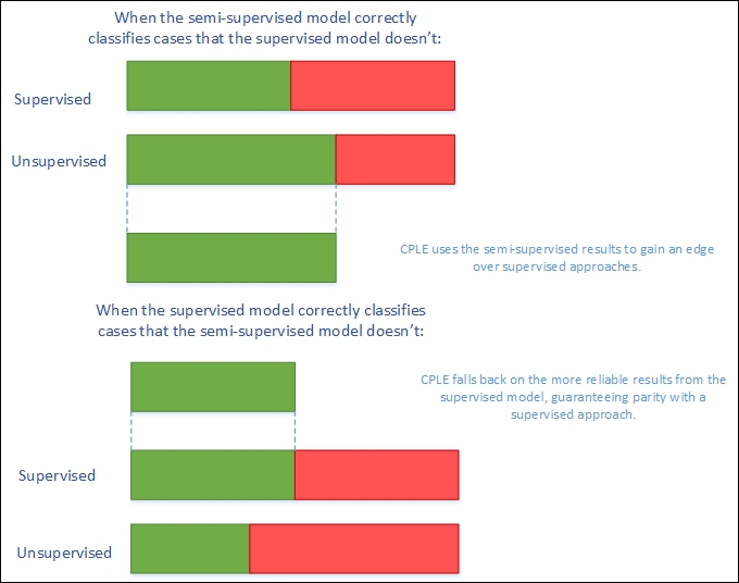
CPLE calculates the relative improvement of any semi-supervised estimate over the supervised solution. Where the supervised solution outperforms the semi-supervised estimate, the loss function shows this and the model can train to adjust the semi-supervised model to reduce this loss. Where the semi-supervised solution outperforms the supervised solution, the model can learn from the semi-supervised model by adjusting model parameters.
However, while this sounds excellent so far, there is a flaw in the theory that has to be addressed. The fact that data labels don't exist for a semi-supervised solution means that the posterior distribution (that CPLE would use to calculate loss) is inaccessible. CPLE's solution to this is to be pessimistic. The CPLE algorithm takes the Cartesian product of all label/prediction combinations and then selects the posterior distribution that minimizes the gain in likelihood.
In real-world machine learning contexts, this is a very safe approach. It delivers the classification accuracy of a supervised approach with semi-supervised performance improvement derived via conservative assumptions. In real applications, these conservative assumptions enable high performance under testing. Even better, CPLE can deliver particular performance improvements on some of the most challenging unsupervised learning cases, where the labeled data is a poor representation of the unlabeled data (by virtue of poor sampling from one or more classes or just because of a shortage of unlabeled cases).
In order to understand how much more effective CPLE can be than semi-supervised or supervised approaches, let's apply the technique to a practical problem. We'll once again work with the semisup-learn library, a specialist Python library, focused on semi-supervised learning, which extends scikit-learn to provide CPLE across any scikit-learn-provided classifier. We begin with a CPLE class:
class CPLELearningModel(BaseEstimator):

    def __init__(self, basemodel, pessimistic=True, predict_from_probabilities = False, use_sample_weighting = True, max_iter=3000, verbose = 1):
        self.model = basemodel
        self.pessimistic = pessimistic
        self.predict_from_probabilities = predict_from_probabilities
        self.use_sample_weighting = use_sample_weighting
        self.max_iter = max_iter
        self.verbose = verbose
We're already familiar with the concept of basemodel. Earlier in this chapter, we employed S3VMs and semi-supervised LDE's. In this situation, we'll again use an LDE; the goal of this first assay will be to try and exceed the results obtained by the semi-supervised LDE from earlier in this chapter. In fact, we're going to blow those results out of the water!
Before we do so, however, let's review the other parameter options. The pessimistic argument gives us an opportunity to use a non-pessimistic (optimistic) model. Instead of following the pessimistic method of minimizing the loss between unlabeled and labeled discriminative likelihood, an optimistic model aims to maximize likelihood. This can yield better results (mostly during training), but is significantly more risky. Here, we'll be working with pessimistic models.
The predict_from_probabilities parameter enables optimization by allowing a prediction to be generated from the probabilities of multiple data points at once. If we set this as true, our CPLE will set the prediction as 1 if the probability we're using for prediction is greater than the mean, or 0 otherwise. The alternative is to use the base model probabilities, which is generally preferable for performance reasons, unless we'll be calling predict across a number of cases.
We also have the option to use_sample_weighting, otherwise known as soft labels (but most familiar to us as posterior probabilities). We would normally take this opportunity, as soft labels enable greater flexibility than hard labels and are generally preferred (unless the model only supports hard class labels).
The first few parameters provide a means of stopping CPLE training, either at maximum iterations or after log-likelihood stops improving (typically because of convergence). The bestdl provides the best discriminative likelihood value and corresponding soft labels; these values are updated on each training iteration:
        self.it = 0
        self.noimprovementsince = 0
        self.maxnoimprovementsince = 3

        self.buffersize = 200
        self.lastdls = [0]*self.buffersize

        self.bestdl = numpy.infty
        self.bestlbls = []


        self.id = str(unichr(numpy.random.randint(26)+97))+str(unichr(numpy.random.randint(26)+97))
The discriminative_likelihood function calculates the likelihood (for discriminative models—that is, models that aim to maximize the probability of a target—y = 1, conditional on the input, X) of an input.
Note
In this case, it's worth drawing your attention to the distinction between generative and discriminative models. While this isn't a basic concept, it can be fundamental in understanding why many classifiers have the goals that they do.
A classification model takes input data and attempts to classify cases, assigning each case a label. There is more than one way to do this.
One approach is to take the cases and attempt to draw a decision boundary between them. Then we can take each new case as it appears and identify which side of the boundary it falls on. This is a discriminative learning approach.
Another approach is to attempt to model the distribution of each class individually. Once a model has been generated, the algorithm can use Bayes' rule to calculate the posterior distribution on the labels given input data. This approach is generative and is a very powerful approach with significant weaknesses (most of which tie into the question of how well we can model our classes). Generative approaches include Gaussian discriminant models (yes, that is a slightly confusing name) and a broad range of Bayesian models. More information, including some excellent recommended reading, is provided in the Further reading section of this chapter.
In this case, the function will be used on each iteration to calculate the likelihood of the predicted labels:
    def discriminative_likelihood(self, model, labeledData, labeledy = None, unlabeledData = None, unlabeledWeights = None, unlabeledlambda = 1, gradient=[], alpha = 0.01):
        unlabeledy = (unlabeledWeights[:, 0]<0.5)*1
        uweights = numpy.copy(unlabeledWeights[:, 0])

        uweights[unlabeledy==1] = 1-uweights[unlabeledy==1]

        weights = numpy.hstack((numpy.ones(len(labeledy)), uweights))
        labels = numpy.hstack((labeledy, unlabeledy))
Having defined this much of our CPLE, we also need to define the fitting process for our supervised model. This uses familiar components, namely, model.fit and model.predict_proba, for probability prediction:
        if self.use_sample_weighting:
            model.fit(numpy.vstack((labeledData, unlabeledData)), labels, sample_weight=weights)
        else:
            model.fit(numpy.vstack((labeledData, unlabeledData)), labels)


        P = model.predict_proba(labeledData)
In order to perform pessimistic CPLE, we need to derive both the labeled and unlabeled discriminative log likelihood. In order, we then perform predict_proba on both the labeled and unlabeled data:
        try:

            labeledDL = -sklearn.metrics.log_loss(labeledy, P)
        except Exception, e:
            print e
            P = model.predict_proba(labeledData)


        unlabeledP = model.predict_proba(unlabeledData)


        try:
            eps = 1e-15
            unlabeledP = numpy.clip(unlabeledP, eps, 1 - eps)
            unlabeledDL = numpy.average((unlabeledWeights*numpy.vstack((1-unlabeledy, unlabeledy)).T*numpy.log(unlabeledP)).sum(axis=1))
        except Exception, e:
            print e
            unlabeledP = model.predict_proba(unlabeledData)
Once we're able to calculate the discriminative log likelihood for both the labeled and unlabeled classification attempts, we can set an objective via the discriminative_likelihood_objective function. The goal here is to use the pessimistic (or optimistic, by choice) methodology to calculate dl on each iteration until the model converges or the maximum iteration count is hit.
On each iteration, a t-test is performed to determine whether the likelihoods have changed. Likelihoods should continue to change on each iteration preconvergence. Sharp-eyed readers may have noticed earlier in the chapter that three consecutive t-tests showing no change will cause the iteration to stop (this is configurable via the maxnoimprovementsince parameter):
        if self.pessimistic:
            dl = unlabeledlambda * unlabeledDL - labeledDL
        else:
            dl = - unlabeledlambda * unlabeledDL - labeledDL

        return dl


    def discriminative_likelihood_objective(self, model, labeledData, labeledy = None, unlabeledData = None, unlabeledWeights = None, unlabeledlambda = 1, gradient=[], alpha = 0.01):
        if self.it == 0:
            self.lastdls = [0]*self.buffersize

        dl = self.discriminative_likelihood(model, labeledData, labeledy, unlabeledData, unlabeledWeights, unlabeledlambda, gradient, alpha)

        self.it += 1
        self.lastdls[numpy.mod(self.it, len(self.lastdls))] = dl

        if numpy.mod(self.it, self.buffersize) == 0: # or True:
            improvement = numpy.mean((self.lastdls[(len(self.lastdls)/2):])) - numpy.mean((self.lastdls[:(len(self.lastdls)/2)]))

            _, prob = scipy.stats.ttest_ind(self.lastdls[(len(self.lastdls)/2):], self.lastdls[:(len(self.lastdls)/2)])

            noimprovement = prob > 0.1 and numpy.mean(self.lastdls[(len(self.lastdls)/2):]) < numpy.mean(self.lastdls[:(len(self.lastdls)/2)])
            if noimprovement:
                self.noimprovementsince += 1
                if self.noimprovementsince >= self.maxnoimprovementsince:

                    self.noimprovementsince = 0
                    raise Exception(" converged.")
            else:
                self.noimprovementsince = 0
On each iteration, the algorithm saves the best discriminative likelihood and the best weight set for use in the next iteration:
        if dl < self.bestdl:
            self.bestdl = dl
            self.bestlbls = numpy.copy(unlabeledWeights[:, 0])

        return dl
One more element worth discussing is how the soft labels are created. We've discussed these earlier in the chapter. This is how they look in code:
f = lambda softlabels, grad=[]: self.discriminative_likelihood_objective(self.model, labeledX, labeledy=labeledy, unlabeledData=unlabeledX, unlabeledWeights=numpy.vstack((softlabels, 1-softlabels)).T, gradient=grad)

lblinit = numpy.random.random(len(unlabeledy))
In a nutshell, softlabels provide a probabilistic version of the discriminative likelihood calculation. In other words, they act as weights rather than hard, binary class labels. Soft labels are calculable using the optimize method:
        try:
            self.it = 0
            opt = nlopt.opt(nlopt.GN_DIRECT_L_RAND, M)
            opt.set_lower_bounds(numpy.zeros(M))
            opt.set_upper_bounds(numpy.ones(M))
            opt.set_min_objective(f)
            opt.set_maxeval(self.max_iter)
            self.bestsoftlbl = opt.optimize(lblinit)
            print " max_iter exceeded."
        except Exception, e:
            print e
            self.bestsoftlbl = self.bestlbls

        if numpy.any(self.bestsoftlbl != self.bestlbls):
            self.bestsoftlbl = self.bestlbls
        ll = f(self.bestsoftlbl)

        unlabeledy = (self.bestsoftlbl<0.5)*1
        uweights = numpy.copy(self.bestsoftlbl)

        uweights[unlabeledy==1] = 1-uweights[unlabeledy==1]

        weights = numpy.hstack((numpy.ones(len(labeledy)), uweights))
labels = numpy.hstack((labeledy, unlabeledy))Once we understand how this works, the rest of the calculation is a straightforward comparison of the best supervised labels and soft labels, setting the bestsoftlabel parameter as the best label set. Following this, the discriminative likelihood is computed against the best label set and a fit function is calculated:
        if self.use_sample_weighting:
            self.model.fit(numpy.vstack((labeledX, unlabeledX)), labels, sample_weight=weights)
        else:
            self.model.fit(numpy.vstack((labeledX, unlabeledX)), labels)

        if self.verbose > 1:
            print "number of non-one soft labels: ", numpy.sum(self.bestsoftlbl != 1), ", balance:", numpy.sum(self.bestsoftlbl<0.5), " / ", len(self.bestsoftlbl)
            print "current likelihood: ", ll
Now that we've had a chance to understand the implementation of CPLE, let's get hands-on with an interesting dataset of our own! This time, we'll change things up by working with the University of Columbia's Million Song Dataset.
The central feature of this algorithm is feature analysis and metadata for one million songs. The data is preprepared and made up of natural and derived features. Available features include things such as the artist's name and ID, duration, loudness, time signature, and tempo of each song, as well as other measures including a crowd-rated danceability score and tags associated with the audio.
This dataset is generally labeled (via tags), but our objective in this case will be to generate genre labels for different songs based on the data provided. As the full million song dataset is a rather forbidding 300 GB, let's work with a 1% (1.8 GB) subset of 10,000 records. Furthermore, we don't particularly need this data as it currently exists; it's in an unhelpful format and a lot of the fields are going to be of little use to us.
The 10000_songs dataset residing in the Chapter 6, Text Feature Engineering folder of our Mastering Python Machine Learning repository is a cleaned, prepared (and also rather large) subset of music data from multiple genres. In this analysis, we'll be attempting to predict genre from the genre tags provided as targets. We'll take a subset of tags as the labeled data used to kick-start our learning and will attempt to generate tags for unlabelled data.
In this iteration, we're going to raise our game as follows:
- Using more labeled data. This time, we'll use 1% of the total dataset size (100 songs), taken at random, as labeled data.
- Using an SVM with a linear kernel as our classifier, rather than the simple linear discriminant analysis we used with our naïve self-training implementation earlier in this chapter.
So, let's get started:
import sklearn.svm
import numpy as np
import random

from frameworks.CPLELearning import CPLELearningModel
from methods import scikitTSVM
from examples.plotutils import evaluate_and_plot

kernel = "linear"

songs = fetch_mldata("10000_songs")
X = songs.data
ytrue = np.copy(songs.target)
ytrue[ytrue==-1]=0

labeled_N = 20
ys = np.array([-1]*len(ytrue))
random_labeled_points = random.sample(np.where(ytrue == 0)[0], labeled_N/2)+
                        random.sample(np.where(ytrue == 1)[0], labeled_N/2)
ys[random_labeled_points] = ytrue[random_labeled_points]
For comparison, we'll run a supervised SVM alongside our CPLE implementation. We'll also run the naïve self-supervised implementation, which we saw earlier in this chapter, for comparison:
basemodel = SGDClassifier(loss='log', penalty='l1') # scikit logistic regression
basemodel.fit(X[random_labeled_points, :], ys[random_labeled_points])
print "supervised log.reg. score", basemodel.score(X, ytrue)


ssmodel = SelfLearningModel(basemodel)
ssmodel.fit(X, ys)
print "self-learning log.reg. score", ssmodel.score(X, ytrue)


ssmodel = CPLELearningModel(basemodel)
ssmodel.fit(X, ys)
print "CPLE semi-supervised log.reg. score", ssmodel.score(X, ytrue)
The results that we obtain on this iteration are very strong:
# supervised log.reg. score 0.698
# self-learning log.reg. score 0.825
# CPLE semi-supervised log.reg. score 0.833
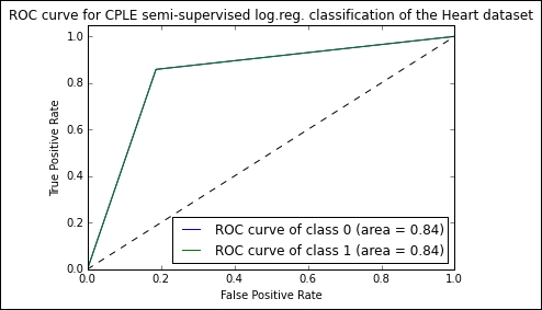
The CPLE semi-supervised model succeeds in classifying with 84% accuracy, a score comparable to human estimation and over 10% higher than the naïve semi-supervised implementation. Notably, it also outperforms the supervised SVM.