
In preceding sections, we've discussed some of the methods by which we might take a dataset and extract a subset of valuable features. These methods have broad applicability but are less helpful when dealing with non-numerical/non-categorical data, or data that cannot be easily translated into numerical or categorical data. In particular, we need to apply different techniques when working with text data.
The techniques that we'll study in this section fall into two main categories—cleaning techniques and feature preparation techniques. These are typically implemented in roughly that order and we'll study them accordingly.
When we work with natural text data, a different set of approaches apply. This is because in real-world contexts, the idea of a naturally clean text dataset is pretty unsafe; text data is rife with misspellings, non-dictionary constructs like emoticons, and in some cases, HTML tagging. As such, we need to be very thorough with our cleaning.
In this section, we'll work with a number of effective text-cleaning techniques, using a pretty gnarly real-world dataset. Specifically, we'll be using the Impermium dataset from a 2012 Kaggle competition, where the competition's goal was to create a model which accurately detects insults in social commentary.
Yes, I do mean Internet troll detection.
Let's get started!
Our first step should be manually checking the input data. This is pretty critical; with text data, one needs to try and understand what issues exist in the data initially so as to identify the cleaning needed.
It's kind of painful to read through a dataset full of hateful Internet commentary, so here's an example entry:
|
ID |
Date |
Comment |
|---|---|---|
|
|
|
|
We have an ID field and date field which don't seem to need much work. The text fields, however, are quite challenging. From this one case, we can already see misspelling and HTML inclusion. Furthermore, many entries in the dataset contain attempts to bypass swear filtering, usually by including a space or punctuation element mid-word. Other data quality issues include multiple vowels (to extend a word), non-ascii characters, hyperlinks... the list goes on.
One option for cleaning this dataset is to use regular expressions, which run over the input data to scrub out data quality issues. However, the quantity and variety of problem formats make it impractical to use a regex-based approach, at least to begin with. We're likely both to miss a lot of cases and also to misjudge the amount of preparation needed, leading us to clean too aggressively, or not aggressively enough; in specific terms we risk cutting into real text content or leaving parts of tags in place. What we need is a solution that will wash out the majority of common data quality problems to begin with so that we can focus on the remaining issues with a script-based approach.
Enter BeautifulSoup. BeautifulSoup is a very powerful text cleaning library which can, among other things, remove HTML markup. Let's take a look at this library in action on our troll data:
from bs4 import BeautifulSoup
import csv

trolls = []
with open('trolls.csv',  'rt') as f:
    reader = csv.DictReader(f)
    for line in reader:
        trolls.append(BeautifulSoup(str(line["Comment"]), "html.parser"))

print(trolls[0])

eg = BeautifulSoup(str(trolls), "html.parser")

print(eg.get_text())|
ID |
Date |
Comments |
|---|---|---|
|
|
|
|
As we can see, we've already made headway on improving the quality of our text data. Yet, it's also clear from these examples that there's a lot of work left to do! As discussed, let's move on to using regular expressions to help further clean and tokenize our data.
Tokenisation is the process of creating a set of tokens from a stream of text. Many tokens are words, while others might be character sets (such as smilies or other punctuation strings, for example, ????????).
Now that we've removed a lot of the HTML ugliness from our initial dataset, we can take steps to further improve the cleanliness of our text data. To do this, we'll leverage the re module, which allows us to use operations over regular expressions, such as substring replacement. We'll perform a series of operations over our input text on this pass, which mostly focus on replacing variable or problematic text elements with tokens. Let's begin with a simple example, replacing e-mail addresses with an _EM token:
text = re.sub(r'[w-][w-.]+@[w-][w-.]+[a-zA-Z]{1,4}', '_EM', text)Similarly, we can remove URLs, replacing them with the _U token:
text = re.sub(r'w+://S+', r'_U', text)
We can automatically remove extra or problematic whitespace and newline characters, hyphens, and underscores. In addition, we'll begin managing the problem of multiple characters, often used for emphasis in informal conversation. Extended series of punctuation characters are encoded here using codes such as _BQ and BX; these longer tags are used as a means of differentiating from the more straightforward _Q and _X tags (which refer to the use of a question mark and exclamation mark, respectively).
We can also use regular expressions to manage extra letters; by cutting down such strings to two characters at most, we're able to reduce the number of combinations to a manageable amount and tokenize that reduced group using the _EL token:
# Format whitespaces
text = text.replace('"', ' ')
text = text.replace(''', ' ')
text = text.replace('_', ' ')
text = text.replace('-', ' ')
text = text.replace('
', ' ')
text = text.replace('\n', ' ')
text = text.replace(''', ' ')
text = re.sub(' +',' ', text)
text = text.replace(''', ' ')


#manage punctuation
text = re.sub(r'([^!?])(?{2,})(|[^!?])', r'1 _BQ
3', text)
text = re.sub(r'([^.])(.{2,})', r'1 _SS
', text)
text = re.sub(r'([^!?])(?|!){2,}(|[^!?])', r'1 _BX
3', text)
text = re.sub(r'([^!?])?(|[^!?])', r'1 _Q
2', text)
text = re.sub(r'([^!?])!(|[^!?])', r'1 _X
2', text)
text = re.sub(r'([a-zA-Z])11+(w*)', r'112 _EL', text)
text = re.sub(r'([a-zA-Z])11+(w*)', r'112 _EL', text)
text = re.sub(r'(w+).(w+)', r'12', text)
text = re.sub(r'[^a-zA-Z]','', text)
Next, we want to begin creating other tokens of interest. One of the more helpful indicators available is the _SW token for swearing. We'll also use regular expressions to help identify and tokenize smileys into one of four buckets; big and happy smileys (_BS), small and happy ones (_S), big and sad ones (_BF), and small and sad ones (_F):
text = re.sub(r'([#%&*$]{2,})(w*)', r'12 _SW', text)


text = re.sub(r' [8x;:=]-?(?:)|}|]|>){2,}', r' _BS', text)
text = re.sub(r' (?:[;:=]-?[)}]d>])|(?:<3)', r' _S', text)
text = re.sub(r' [x:=]-?(?:(|[|||\|/|{|<){2,}', r' _BF', text)
text = re.sub(r' [x:=]-?[([|\/{<]', r' _F', text)
Note
Smileys are complicated by the fact that their uses change frequently; while this series of characters is reasonably current, it's by no means complete; for example, see emojis for a range of non-ascii representations. For several reasons, we'll be removing non-ascii text from this example (a similar approach is to use a dictionary to force compliance), but both approaches have the obvious drawback that they remove cases from the dataset, meaning that any solution will be imperfect. In some cases, this approach may lead to the removal of a substantial amount of data. In general, then, it's prudent to be aware of the general challenge around character-based images in text content.
Following this, we want to begin splitting text into phrases. This is a simple application of str.split, which enables the input to be treated as a vector of words (words) rather than as long strings (re):
phrases = re.split(r'[;:.()
]', text)
phrases = [re.findall(r'[w%*&#]+', ph) for ph in phrases]
phrases = [ph for ph in phrases if ph]

words = []

for ph in phrases:
      words.extend(ph)
This gives us the following:
|
ID |
Date |
Comments |
|---|---|---|
|
|
|
|
Next, we perform a search for single-letter sequences. Sometimes, for emphasis, Internet communication involves the use of spaced single-letter chains. This may be attempted as a method of avoiding curse word detection:
tmp = words
words = []
new_word = ''
for word in tmp:
   if len(word) == 1:
      new_word = new_word + word
   else:
      if new_word:
         words.append(new_word)
         new_word = ''
      words.append(word)
So far, then, we've gone a long way toward cleaning and improving the quality of our input data. There are still outstanding issues, however. Let's reconsider the example we began with, which now looks like the following:
|
ID |
Date |
Words |
|---|---|---|
|
|
|
|
Much of our early cleaning has passed this example by, but we can see the effect of vectorising the sentence content as well as the now-cleaned HTML tags. We can also see that the emote used has been captured via the _F tag. When we look at a more complex test case, we see even more substantial change results:
|
Raw |
Cleaned and split |
|---|---|
|
|
|
However, there are two significant problems still obvious in both examples. In the first case, we have a misspelled word; we need to find a way to eliminate this. Secondly, a lot of the words in both examples (for example. are, pm) aren't terribly informative in and of themselves. The problem we find, particularly for shorter text samples, is that what's left after cleaning may contain only one or two meaningful terms. If these terms are not terribly common in the corpus as a whole, it can prove to be very difficult to train a classifier to recognise these terms' significance.
I expect that we all know that English language words come in several types—nouns, verbs, adverbs, and so on. These are commonly referred to as parts of speech. If we know that a certain word is an adjective, as opposed to a verb or stop word (such as a, the, or of), we can treat it differently or more importantly, our algorithm can!
If we can perform part of speech tagging by identifying and encoding word classes as categorical variables, we're able to improve the quality of our data by retaining only the valuable content. The full range of text tagging options and techniques is too broad to be effectively covered in one section of this chapter, so we'll look at a subset of the applicable tagging techniques. Specifically, we'll focus on n-gram tagging and backoff taggers, a pair of complimentary techniques that allow us to create powerful recursive tagging algorithms.
We'll be using a Python library called the Natural Language Toolkit (NLTK). NLTK offers a wide array of functionality and we'll be relying on it at several points in this chapter. For now, we'll be using NLTK to perform tagging and removal of certain word types. Specifically, we'll be filtering out stop words.
To answer the obvious first question (why eliminate stop words?), it tends to be true that stop words add little to nothing to most text analysis and can be responsible for a degree of noise and training variance. Fortunately, filtering stop words is pretty straightforward. We'll simply import NLTK, download and import the dictionaries, then perform a scan over all words in our pre-existing word vector, removing any stop words found:
import nltk
nltk.download()
from nltk.corpus import stopwords

words = [w for w in words if not w in stopwords.words("english")]
I'm sure you'll agree that this was pretty straightforward! Let's move on to discuss more NLTK functionality, specifically, tagging.
Tagging is the process of identifying parts of speech, as we described previously, and applying tags to each term.
In its simplest form, tagging can be as straightforward as applying a dictionary over our input data, just as we did previously with stopwords:
tagged = ntlk.word_tokenize(words)
However, even brief consideration will make it obvious that our use of language is a lot more complicated than this allows. We may use a word (such as ferry) as one of several parts of speech and it may not be straightforward to decide how to treat each word in every utterance. A lot of the time, the correct tag can only be understood contextually given the other words and their positioning within the phrase.
Thankfully, we have a number of useful techniques available to help us solve linguistic challenges.
A sequential tagging algorithm is one that works by running through the input dataset, left-to-right and token-by-token (hence sequential!), tagging each token in succession. The decision over which token to assign is made based on that token, the tokens that preceded it, and the predicted tags for those preceding tokens.
In this section, we'll be using an n-gram tagger. An n-gram tagger is a type of sequential tagger, which is pretrained to identify appropriate tags. The n-gram tagger takes (n-1)-many preceding POS tags and the current token into consideration in producing a tag.
Note
For clarity, an n-gram is the term used for a contiguous sequence of n-many elements from a given set of elements. This may be a contiguous sequence of letters, words, numerical codes (for example, for state changes), or other elements. N-grams are widely used as a means of capturing the conjunct meaning of sets of elements—be those phrases or encoded state transitions—using n-many elements.
The simplest form of n-gram tagger is one where n = 1, referred to as a unigram tagger. A unigram tagger operates quite simply, by maintaining a conditional frequency distribution for each token. This conditional frequency distribution is built up from a training corpus of terms; we can implement training using a helpful train method belonging to the NgramTagger class in NLTK. The tagger assumes that the tag which occurs most frequently for a given token in a given sequence is likely to be the correct tag for that token. If the term
carp is in the training corpus as a noun four times and as a verb twice, a unigram tagger will assign the noun tag to any token whose type is carp.
This might suffice for a first-pass tagging attempt but clearly, a solution that only ever serves up one tag for each set of homonyms isn't always going to be ideal. The solution we can tap into is using n-grams with a larger value of n. With n = 3 (a trigram tagger), for instance, we can see how the tagger might more easily distinguish the input He tends to carp on a lot from He caught a magnificent carp!
However, once again there is a trade-off here between accuracy of tagging and ability to tag. As we increase n, we're creating increasingly long n-grams which become increasingly rare. In a very short time, we end up in a situation where our n-grams are not occurring in the training data, causing our tagger to be unable to find any appropriate tag for the current token!
In practice, we find that what we need is a set of taggers. We want our most reliably accurate tagger to have the first shot at trying to tag a given dataset and, for any case that fails, we're comfortable with having a more reliable but potentially less accurate tagger have a try.
Happily, what we want already exists in the form of backoff tagging. Let's find out more!
Sometimes, a given tagger may not perform reliably. This is particularly common when the tagger has high accuracy demands and limited training data. At such times, we usually want to build an ensemble structure that lets us use several taggers simultaneously.
To do this, we create a distinction between two types of taggers: subtaggers and backoff taggers. Subtaggers are taggers like the ones we saw previously, sequential and Brill taggers. Tagging structures may contain one or multiple of each kind of tagger.
If a subtagger is unable to determine a tag for a given token, then a backoff tagger may be referred to instead. A backoff tagger is specifically used to combine the results of an ensemble of (one or more) subtaggers, as shown in the following example diagram:

In simple implementations, the backoff tagger will simply poll the subtaggers in order, accepting the first none-null tag provided. If all subtaggers return null for a given token, the backoff tagger will assign a none tag to that token. The order can be determined.
Backoffs are typically used with multiple subtaggers of different types; this enables a data scientist to harness the benefits of multiple types of tagger simultaneously. Backoffs may refer to other backoffs as needed, potentially creating highly redundant or sophisticated tagging structures:
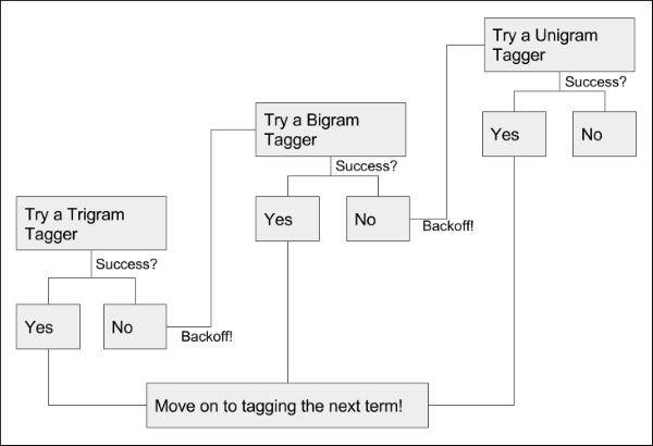
In general terms, backoff taggers provide redundancy and enable you to use multiple taggers in a composite solution. To solve our immediate problem, let's implement a nested series of n-gram taggers. We'll start with a trigram tagger, which will use a bigram tagger as its backoff tagger. If neither of these taggers has a solution, we'll have a unigram tagger as an additional backoff. This can be done very simply, as follows:
brown_a = nltk.corpus.brown.tagged_sents(categories= 'a')

tagger = None
for n in range(1,4):
  tagger = NgramTagger(n, brown_a, backoff = tagger)

words  = tagger.tag(words)
Once we've engaged in well-thought-out text cleaning practices, we need to take additional steps to ensure that our text becomes useful features. In order to do this, we'll look at another set of staple techniques in NLP:
- Stemming
- Lemmatising
- Bagging using random forests
Another challenge when working with linguistic datasets is that multiple word forms exist for many word stems. For example, the root dance is the stem of multiple other words—dancing, dancer, dances, and so on. By finding a way to reduce this plurality of forms into stems, we find ourselves able to improve our n-gram tagging and apply new techniques such as lemmatisation.
The techniques that enable us to reduce words to their stems are called stemmers. Stemmers work by parsing words as consonant/vowel strings and applying a series of rules. The most popular stemmer is the porter stemmer, which works by performing the following steps;
- Simplifying the range of suffixes by reducing (for example, ies becomes i) to a smaller set.
- Removing suffixes in several passes, with each pass removing a set of suffix types (for example, past particple or plural suffixes such as ousness or alism).
- Once all suffixes are removed, cleaning up word endings by adding 'e's where needed (for example, ceas becomes cease).
- Removing double 'l's.
The porter stemmer works very effectively. In order to understand exactly how well it works, let's see it in action!
from nltk.stem import PorterStemmer

stemmer = PorterStemmer()

stemmer.stem(words)
The output of this stemmer, as demonstrated on our pre-existing example, is the root form of the word. This may be a real word, or it may not; dancing, for instance, becomes danci. This is okay, but it's not really ideal. We can do better than this!
To consistently reach a real word form, let's apply a slightly different technique, lemmatisation. Lemmatisation is a more complex process to determine word stems; unlike porter stemming, it uses a different normalisation process for different parts of speech. Unlike Porter Stemming it also seeks to find actual roots for words. Where a stem does not have to be a real word, a lemma does. Lemmatization also takes on the challenge of reducing synonyms down to their roots. For example, where a stemmer might turn the term books into the term book, it isn't equipped to handle the term tome. A lemmatizer can process both books and tome, reducing both terms to book.
As a necessary prerequisite, we need the POS for each input token. Thankfully, we've already applied a POS tagger and can work straight from the results of that process!
from nltk.stem import PorterStemmer, WordNetLemmatizer

lemmatizer = WordNetLemmatizer()

words = lemmatizer.lemmatize(words, pos = 'pos')
The output is now what we'd expect to see:
|
Source Text |
Post-lemmatisation |
|---|---|
|
|
|
We've now successfully stemmed our input text data, massively improving the effectiveness of lookup algorithms (such as many dictionary-based approaches) in handling this data. We've removed stop words and tokenized a range of other noise elements with regex methods. We've also removed any HTML tagging. Our text data has reached a reasonably processed state. There's one more linchpin technique that we need to learn, which will let us generate features from our text data. Specifically, we can use bagging to help quantify the use of terms.
Let's find out more!
Bagging is part of a family of techniques that may collectively be referred to as subspace methods. There are several forms of method, with each having a separate name. If we draw random subsets from the sample cases, then we're performing pasting. If we're sampling from cases with replacement, it's referred to as bagging. If instead of drawing from cases, we work with a subset of features, then we're performing attribute bagging. Finally, if we choose to draw from both sample cases and features, we're employing what's known as a random patches technique.
The feature-based techniques, attribute bagging, and Random Patch methods are very valuable in certain contexts, particularly very high-dimensional ones. Medical and genetics contexts both tend to see a lot of extremely high-dimensional data, so feature-based methods are highly effective within those contexts.
In NLP contexts, it's common to work with bagging specifically. In the context of linguistic data, what we'll be dealing with is properly called a bag of words. A bag of words is an approach to text data preparation that works by identifying all of the distinct words (or tokens) in a dataset and then counting their occurrence in each sample. Let's begin with a demonstration, performed over a couple of example cases from our dataset:
|
ID |
Date |
Words |
|---|---|---|
|
|
|
|
|
|
|
|
This gives us the following 12-part list of terms:
[
  "_F"
  "how"
  "are"
  "you"
  "not"
  "ded"
  "living"
  "proof"
  "that"
  "bath"
  "salts"
  "effect"
  "thinking"
]
Using the indices of this list, we can create a 12-part vector for each of the preceding sentences. This vector's values are filled by traversing the preceding list and counting the number of times each term occurs for each sentence in the dataset. Given our pre-existing example sentences and the list we created from them, we end up creating the following bags:
|
ID |
Date |
Comment |
Bag of words |
|---|---|---|---|
|
|
|
|
|
|
|
|
|
|
This is the core of a bag of words implementation. Naturally, once we've translated the linguistic content of text into numerical vectors, we're able to start using techniques that add sophistication to how we use this text in classification.
One option is to use weighted terms. We can use a term weighting scheme to modify the values within each vector so that terms that are indicative or helpful for classification are emphasized. Weighting schemes may be straightforward masks, such as a binary mask that indicates presence versus absence.
Binary masking can be useful if certain terms are used much more frequently than normal; in such cases, specific scaling (for example, log-scaling) may be needed if a binary mask is not used. At the same time, though, frequency of term use can be informative (it may indicate emphasis, for instance) and the decision over whether to apply a binary mask is not always made simply.
Another weighting option is term frequency-inverse document frequency, or tf-idf. This scheme compares frequency of usage within a specific sentence and the dataset as a whole and uses values that increase if a term is used more frequently within a given sample than within the whole corpus.
Variations on tf-idf are frequently used in text mining contexts, including search engines. Scikit-learn provides a tf-idf implementation, TfidfVectoriser, which we'll shortly use to employ tf-idf for ourselves.
Now that we have an understanding of the theory behind bag of words and can see the range of technical options available to us once we develop vectors of word use, we should discuss how a bag of words implementation can be undertaken. Bag of words can be easily applied as a wrapper to a familiar model. While in general, subspace methods may use any of a range of base models (SVMs and linear regression models are common), it is very common to use random forests in a bag of words implementation, wrapping up preparation and learning into a concise script. In this case, we'll employ bag of words independently for now, saving classification via a random forest implementation for the next section!
Note
While we'll discuss random forests in greater detail in Chapter 8, Ensemble Methods, (which describes the various types of ensemble that we can create), it is helpful for now to note that a random forest is a set of decision trees. They are powerful ensemble models that are created either to run in parallel (yielding a vote or other net outcome) or boost one another (by iteratively adding a new tree to model the parts of the solution that the pre-existing set of trees couldn't model well).
Due to the power and ease of use of random forests, they are commonly used as benchmarking algorithms.
The process of implementing bag of words is, again, fairly straightforward. We initialize our bagging tool (matter-of-factly referred to as a vectorizer). Note that for this example, we're putting a limit on the size of the feature vector. This is largely to save ourselves some time; each document must be compared against each item in the feature list, so when we get to running our classifier this could take a little while!
from sklearn.feature_extraction.text import TfidfVectorizer

vectorizer = TfidfVectorizer(analyzer = "word",
                             tokenizer = None,
                             preprocessor = None,
                             stop_words = None,
                             max_features = 5000)
Our next step is to fit the vectorizer on our word data via fit_transform; as part of the fitting process, our data is transformed into feature vectors:
train_data_features = vectorizer.fit_transform(words)

train_data_features = train_data_features.toarray()
This completes the pre-processing of our text data. We've taken this dataset through a full battery of text mining techniques, walking through the theory and reasoning behind each technique as well as employing some powerful Python scripts to process our test dataset.We're in a good position now to take a crack at Kaggle's insult detection challenge!
So, now that we've done some initial preparation of the dataset, let's give the real problem a shot and see how we do. To help set the scene, let's consider Impermium's guidance and data description:
This is a single-class classification problem. The label is either 0 meaning a neutral comment, or 1 meaning an insulting comment (neutral can be considered as not belonging to the insult class. Your predictions must be a real number in the range [0,1] where 1 indicates 100% confident prediction that comment is an insult.
- We are looking for comments that are intended to be insulting to a person who is a part of the larger blog/forum conversation.
- We are NOT looking for insults directed to non-participants (such as celebrities, public figures etc.).
- Insults could contain profanity, racial slurs, or other offensive language. But often times, they do not.
- Comments which contain profanity or racial slurs, but are not necessarily insulting to another person are considered not insulting.
- The insulting nature of the comment should be obvious, and not subtle.
- There may be a small amount of noise in the labels as they have not been meticulously cleaned. However, contestants can be confident the error in the training and testing data is < 1%.
Contestants should also be warned that this problem tends to strongly overfit. The provided data is generally representative of the full test set, but not exhaustive by any measure. Impermium will be conducting final evaluations based on an unpublished set of data drawn from a wide sample.
This is pretty nice guidance, in that it raises two particular points of caution. The desired score is the area under the curve (AUC), which is a measure that is very sensitive both to false positives and to incorrect negative results (specificity and sensitivity).
The guidance clearly states that continuous predictions are desired rather than binary 0/1 outputs. This becomes critically important when using AUC; even a small amount of incorrect predictions given will radically decrease one's score if you only use categorical values. This suggests that rather than using the RandomForestClassifier algorithm, we'll want to use the RandomForestRegressor, a regression-focused alternative, and then rescale the results between zero and one.
Real Kaggle contests are run in a much more challenging and realistic environment—one where the correct solution is not available. In Chapter 8, Ensemble Methods, we'll explore how top data scientists react and thrive in such environments. For now, we'll take advantage of having the ability to confirm whether we're doing well on the test dataset. Note that this advantage also presents a risk; if the problem overfits strongly, we'll need to be disciplined to ensure that we're not overtraining on the test data!
In addition, we also have the benefit of being able to see how well real contestants did. While we'll save the real discussion for Chapter 8, Ensemble Methods, it's reasonable to expect each highly-ranking contestant to have submitted quite a large number of failed attempts; having a benchmark will help us tell whether we're heading in the right direction.
Specifically, the top 14 participants on the private (test) leaderboard managed to reach an AUC score of over 0.8. The top scorer managed a pretty impressive 0.84, while over half of the 50 teams who entered scored above 0.77.
As we discussed earlier, let's begin with a random forest regression model.
Note
A random forest is an ensemble of decision trees.
While a single decision tree is likely to suffer from variance- or bias-related issues, random forests are able to use a weighted average over multiple parallel trials to balance the results of modeling.
Random forests are very straightforward to apply and are a good first-pass technique for a new data challenge; applying a random forest classifier to the data early on enables you to develop a good understanding as to what initial, baseline classification accuracy will look like as well as giving valuable insight into how the classification boundaries were formed; during the initial stages of working with a dataset, this kind of insight is invaluable.
Scikit-learn provides RandomForestClassifier to enable the easy application of a random forest algorithm.
For this first pass, we'll use 100 trees; increasing the number of trees can improve classification accuracy but will take additional time. Generally speaking, it's sensible to attempt fast iteration in the early stages of model creation; the faster you can repeatedly run your model, the faster you can learn what your results are looking like and how to improve them!
We begin by initializing and training our model:
trollspotter = RandomForestRegressor(n_estimators = 100, max_depth = 10, max_features = 1000)

y = trolls["y"]

trollspotted = trollspotter.fit(train_data_features, y)
We then grab the test data and apply our model to predict a score for each test case. We rescale these scores using a simple stretching technique:
moretrolls = pd.read_csv('moretrolls.csv', header=True, names=['y', 'date', 'Comment', 'Usage'])
moretrolls["Words"] = moretrolls["Comment"].apply(cleaner)

y = moretrolls["y"]

test_data_features = vectorizer.fit_transform(moretrolls["Words"])
test_data_features = test_data_features.toarray()

pred = pred.predict(test_data_features)
pred = (pred - pred.min())/(pred.max() - pred.min())
Finally, we apply the roc_auc function to calculate an AUC score for the model:
fpr, tpr, _ = roc_curve(y, pred)
roc_auc = auc(fpr, tpr)
print("Random Forest benchmark AUC score, 100 estimators")
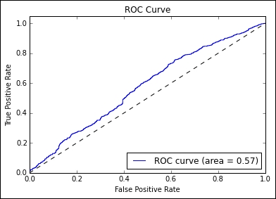
print(roc_auc)As we can see, the results are definitely not at the level that we want them to be at:
Random Forest benchmark AUC score, 100 estimators
0.537894912105
Thankfully, we have a number of options that we can try to configure here:
- Our approach to how we work with the input (preprocessing steps and normalisation)
- The number of estimators in our random forest
- The classifier we choose to employ
- The properties of our bag of words implementation (particularly the maximum number of terms)
- The structure of our n-gram tagger
On our next pass, let's adjust the size of our bag of words implementation, increasing the term cap from a slightly arbitrary 5,000 to anywhere up to 8,000 terms; rather than picking just one value, we'll run over a range and see what we can learn. We'll also increase the number of trees to a more reasonable number (in this case, we stepped up to 1000):
Random Forest benchmark AUC score, 1000 estimators
0.546439310772
These results are slightly better than the previous set, but not dramatically so. They're definitely a fair distance from where we want to be! Let's go further and set up a different classifier. Let's try a fairly familiar option—the SVM. We'll set up our own SVM object to work with:
class SVM(object):

    def __init__(self, texts, classes, nlpdict=None):

        self.svm = svm.LinearSVC(C=1000, class_weight='auto')
        if nlpdict:
            self.dictionary = nlpdict
        else:
            self.dictionary = NLPDict(texts=texts)
        self._train(texts, classes)

    def _train(self, texts, classes):
        vectors = self.dictionary.feature_vectors(texts)
        self.svm.fit(vectors, classes)

    def classify(self, texts):
        vectors = self.dictionary.feature_vectors(texts)
        predictions = self.svm.decision_function(vectors)
        predictions = p.transpose(predictions)[0:len(predictions)]
        predictions = predictions / 2 + 0.5
        predictions[predictions > 1] = 1
        predictions[predictions < 0] = 0
        return predictions
While the workings of SVM are almost impenetrable to human assessment, as an algorithm it operates effectively, iteratively translating the dataset into multiple additional dimensions in order to create complex hyperplanes at optimal class boundaries. It isn't a huge surprise, then, to see that the quality of our classification has increased:
SVM AUC score
0.625245653817
Perhaps we're not getting enough visibility into what's happening with our results. Let's try shaking things up with a different take on performance measurement. Specifically, let's look at the difference between the model's label predictions and actual targets to see whether the model is failing more frequently with certain types of input.
So we've taken our prediction quite far. While we still have a number of options on the table, it's worth considering the use of a more sophisticated ensemble of models as being a solid option. In this case, leveraging multiple models instead of just one can enable us to obtain the relative advantages of each. To try out an ensemble against this example, run the score_trolls_blendedensemble.py script.
Note
This ensemble is a blended/stacked ensemble. We'll be spending more time discussing how this ensemble works in Chapter 8, Ensemble Methods!
Plotting our results, we can see that performance has improved, but by significantly less than we'd hoped:
We're clearly having some issues with building a model against this data, but at this point, there isn't a lot of value in throwing a more developed model at the problem. We need to go back to our features and aim to extend the feature set.
At this point, it's worth taking some pointers from one of the most successful entrants of this particular Kaggle contest. In general, top-scoring entries tend to be developed by finding all of the tricks around the input data. The second-place contestant in the official Kaggle contest that this dataset was drawn from was a user named tuzzeg. This contestant provided a usable code repository at https://github.com/tuzzeg/detect_insults.
Tuzzeg's implementation differs from ours by virtue of much greater thoroughness. In addition to the basic features that we built using POS tagging, he employed POS-based bigrams and trigrams as well as subsequences (created from sliding windows of N-many terms). He worked with n-grams up to 7-grams and created character n-grams of lengths 2, 3, and 4.
Furthermore, tuzzeg took the time to create two types of composite model, both of which were incorporated into his solution—sentence level and ranking models. Ranking took our rationalization around the nature of the problem a step further by turning the cases in our data into ranked continuous values.
Meanwhile, the innovative sentence-level model that he developed was trained specifically on single-sentence cases in the training data. For prediction on test data, he split the cases into sentences, evaluated each separately, and took only the highest score for sentences within the case. This was to accommodate the expectation that in natural language, speakers will frequently confine insulting comments to a single part of their speech.
Tuzzeg's model created over 100 feature groups (where a stem-based bigram is an example feature group—a group in the sense that the bigram process creates a vector of features), with the most important ones (ranked by impact) being the following:
stem subsequence based         0.66
stem based (unigrams, bigrams) 0.18
char ngrams based (sentence)   0.07
char ngrams based              0.04
all syntax                     0.006
all language models            0.004
all mixed                      0.002
This is interesting, in that it suggests that a set of feature translations that we aren't currently using is important in generating a usable solution. Particularly, the subsequence-based features are only a short step from our initial feature set, making it straightforward to add the extra feature:
def subseq2(n, xs):
  l = len(xs)
  return ['%s %s' % (xs[i], xs[j]) for i in xrange(l-1) for j in xrange(i+1, i+n+1) if j < l]

def getSubseq2(seqF, n):
  def f(row):
    seq = seqF(row)
    return set(seq + subseq2(n, seq))
  return f

Subseq2test = getSubseq2(line, 2)
This approach yields excellent results. While I'd encourage you to export Tuzzeg's own solution and apply it, you can also look at the score_trolls_withsubseq.py script provided in this project's repository to get a feeling for how powerful additional features can be incorporated.
With these additional features added, we see a dramatic improvement in our AUC score:
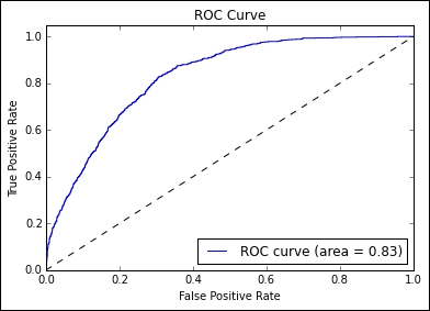
Running this code provides a very healthy 0.834 AUC score. This simply goes to show the power of thoughtful and innovative feature engineering; while the specific features generated in this chapter will serve you well in other contexts, specific hypotheses (such as hostile comments being isolated to specific sentences within a multi-sentence comment) can lead to very effective features.
As we've had the luxury of checking our reasoning against test data throughout this chapter, we can't reasonably say that we've worked under life-like conditions. We didn't take advantage of having access to the test data by reviewing it ourselves, but it's fair to say that knowing what the private leaderboard scored for this challenge made it easier for us to target the right fixes. In Chapter 8, Ensemble Methods, we'll be working on another tricky Kaggle problem in a more rigorous and realistic way. We'll also be discussing ensembles in depth!