
The most important factor involved in successful machine learning is the quality of your input data. A good model with misleading, inappropriately normalized, or uninformative data will not see the same level of success anywhere near a model run over appropriately prepared data.
In some cases, you have the ability to specify data collection or have access to a useful, sizeable, and varied set of source data. With the right knowledge and skillset, you can use this data to create highly useful feature sets.
In general, having a strong knowledge as to how to construct good feature sets is very helpful as it enables you to audit and assess any new dataset for missed opportunities. In this chapter, we will introduce a design process and technique set that make it easier to create effective feature sets.
As such, we'll begin by discussing some techniques that we can use to extend or reinterpret existing features, potentially creating a large number of useful parameters to include in our models.
However, as we will see, there are limitations on the effective use of feature engineering techniques and we need to be mindful of the risks around engineered datasets.
We have discussed what you can do about patching up data quality issues in your data and we have talked about how you can creatively use dimensions in what you have to join to external data.
Once you have a reasonably well-understood and quality-checked set of data in front of you, there is usually still a significant amount of work needed before you can produce effective models from that data.
The main challenge with directly feeding unprepared data to many machine learning models is that the algorithm is sensitive to the relative size of different variables. If your dataset has multiple parameters whose ranges differ, some algorithms will treat the variables whose variance is greater as indicative of more significant change than algorithms with smaller values and less variance.
The key to resolving this potential problem is rescaling, a process by which parameter values' relative size is adjusted while retaining the initial ordering of values within each parameter (a monotonic translation).
Gradient descent algorithms (which include most deep learning algorithms—http://sebastianruder.com/optimizing-gradient-descent/) are significantly more efficient if the input data is scaled prior to training. To understand why, we'll resort to drawing some pictures. A given series of training steps may appear as follows:
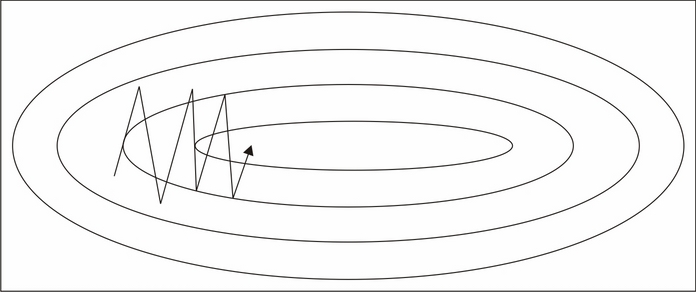
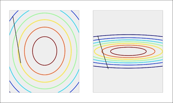
When applied to unscaled data, these training steps may not converge effectively (as per the left-hand example in the following diagram).
With each parameter having a differing scale, the parameter space in which models are attempting to train can be highly distorted and complex. The more complex this space, the harder it becomes to train a model within it. This is an involved subject that can be effectively described, in general terms, through a metaphor, but for readers looking for a fuller explanation there is an excellent reference in this chapter's Further reading section. For now, it is not unreasonable to think in terms of gradient descent models during training as behaving like marbles rolling down a slope. These marbles are prone to getting stuck in saddle points or other complex geometries on the slope (which, in this context, is the surface created by our model's objective function—the learning function whose output our models typically train to minimize). With scaled data, however, the surface becomes more regularly-shaped and training can become much more effective:
The classic example is a linear rescaling between 0 and 1; with this method, the largest parameter value is rescaled to 1, the smallest to 0, with intermediate values falling in the 0-1 interval, proportionate to their original size relative to the largest and smallest values. Under such a transformation, the vector [0,10,25,20,18], for instance, would become [0,0.4, 1, 0.8, 0.72].
The particular value of this transformation is that, for multiple data points that may vary in magnitude in its raw form, the rescaled features will sit within the same range, enabling your machine learning algorithm to train on meaningful information content.
This is the most straightforward rescaling option, but there are some nonlinear scaling alternatives that can be much more helpful in the right circumstances; these include square scaling, square root scaling, and perhaps most commonly, log-scaling.
Log-scaling of parameter values is very common in physics and in contexts where the underlying data is frequently affected by a power law (for example, an exponential growth in y given a linear increase in x).
Unlike linear rescaling, log-scaling adjusts the relative spacing between data cases. This can be a double-edged sword. On the one hand, log-scaling handles outlying cases very well. Let's take an example dataset describing individual net wealth for members of a fictional population, described by the following summary statistics:
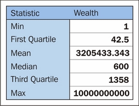
Prior to rescaling, this population is hugely skewed toward that single individual with absurd net worth. The distribution of cases per decile is as follows:
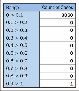
After log-scaling, this distribution is far friendlier:
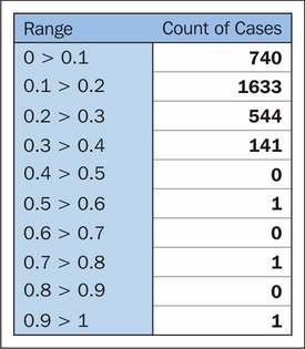
We could've chosen to take scaling further and drawn out the first half of this distribution more by doing that. In this case, log-10 normalization significantly reduces the impact of these outlying values, enabling us to retain outliers in the dataset without losing detail at the lower end.
With this said, it's important to note that in some contexts, that same enhancement of clustered cases can enhance noise in variant parameter values and create the false impression of greater spacing between values. This tends not to negatively affect how log-scaling handles outliers; the impact is usually seen for groups of smaller-valued cases whose original values are very similar.
The challenges created by introducing nonlinearities through log-scaling are significant and in general, nonlinear scaling is only recommended for variables that you understand and have a nonlinear relationship or trend underlying them.
Rescaling is a standard part of preprocessing in many machine learning applications (for instance, almost all neural networks). In addition to rescaling, there are other preparatory techniques, which can improve model performance by strategically reducing the number of parameters input to the model. The most common example is of a derived measure that takes multiple existing data points and represents them within a single measure.
These are extremely prevalent; examples include acceleration (as a function of velocity values from two points in time), body mass index (as a function of height, weight, and age), and price-earnings (P/E) ratio for stock scoring. Essentially, any derived score, ratio, or complex measure that you ever encounter is a combination score formed from multiple components.
For datasets in familiar contexts, many of these pre-existing measures will be well-known. Even in relatively well-known areas, however, looking for new supporting measures or transformations using a mix of domain knowledge and existing data can be very effective. When thinking through derived measure options, some useful concepts are as follows:
- Two variable combinations: Multiplication, division, or normalization of the n parameter as a function of the m parameter.
- Measures of change over time: A classic example here is acceleration or 7D change in a measure. In more complex contexts, the slope of an underlying time series function can be a helpful parameter to work with instead of working directly with the current and past values.
- Subtraction of a baseline: Using a base expectation (a flat expectation such as the baseline churn rate) to recast a parameter in terms of that baseline can be a more immediately informative way of looking at the same variable. For the churn example, we could generate a parameter that describes churn in terms of deviation from an expectation. Similarly, in stock trading cases, we might look at closing price in terms of the opening price.
- Normalization: Following on from the previous case, normalization of parameter values based on the values of another parameter or baseline that is dynamically calculated given properties of other variables. One example here is failed transaction rate; in addition to looking at this value as a raw (or rescaled) count, it often makes sense to normalize this in terms of attempted transactions.
Creative recombination of these different elements lets us build very effective scores. Sometimes, for instance, a parameter that tells us the slope of customer engagement (declining or increasing) over time needs to be conditioned on whether that customer was previously highly engaged or hardly engaged, as a slight decline in engagement might mean very different things in each context. It is the data scientist's job to effectively and creatively feature sets that capture these subtleties for a given domain.
So far, this discussion has focused on numerical data. Often, however, useful data is locked up inside non-numeric parameters such as codes or categorical data. Accordingly, we will next discuss a set of effective techniques to turn non-numeric features into usable parameters.
A common challenge, which can be problematic and problem-specific, is how non-numeric features are treated. Frequently, valuable information is encoded within non-numerical shorthand values. In the case of stock trades, for instance, the identity of the stock itself (for example, AAPL) as well as that of the buyer and seller is interesting information that we expect to relate meaningfully to our problem. Taking this example further, we might also expect some stocks to trade differently from others even within the industry, and organizational differences within companies, which may occur at some or all points of time, also provide important context.
One simple option that works in some cases is building an aggregation or series of aggregations. The most obvious example is a count of occurrences with the possibility of creating extended measures (changes in count between two time windows) as described in the preceding section.
Building summary statistics and reducing the number of rows in the dataset introduces the risk of reducing the amount of information that your model has available to learn from (increasing the risk of model fragility and overfitting). As such, it's generally a bad idea to extensively aggregate and reduce input data. This is doubly true with deep learning techniques, such as the algorithms discussed and used in Chapters 2-4.
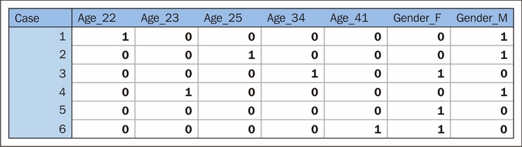
Rather than extensively using aggregation-based approaches, let's look at an alternative way of translating string-encoded values into numerical data. Another very popular class of techniques is encoding, with the most common encoding tactic being one-hot encoding. One-hot encoding is the process of turning a series of categorical responses (for example, age groups) into a set of binary variables, with each response option (for example, 18-30) represented by its own binary variable. This is a little more intuitive when presented visually:
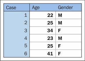
After encoding, this dataset of categorical and continuous variables becomes a tensor of binary variables:
The advantage that this presents is significant; it enables us to tap into the very valuable tag information contained within a lot of datasets without aggregation or risk of reducing the information content of the data. Furthermore, one-hot allows us to separate specific response codes for encoded variables into separate features, meaning that we can identify more or less meaningful codes for a specific variable and only retain the important values.
Another very effective technique, used primarily for text codes, is known as the hash trick. A hash, in simple terms, is a function that translates data into a numeric representation. Hashes will be a familiar concept to many, as they're frequently used to encode sensitive parameters and summarize otherwise bulky data. In order to get the most out of the hash trick, however, it's important to understand how the trick works and what can be done with it.
We can use hashing to turn a text phrase into a numeric value that we can use as an identifier for that phrase. While there are many applications of different hashing algorithms, in this context even a simple hash makes it straightforward to turn string keys and codes into numerical parameters that we can model effectively.
A very simple hash might turn each alphabet character into a corresponding number. a would become 1, b would be 2, and so on. Hashes could be generated for words and phrases by summing those values. The phrase cat gifs would translate under this scheme as follows:
Cat: 3 + 1 + 20
Gifs: 7 + 9 + 6 + 19
Total: 65
This is a terrible hash for two reasons (quite disregarding the fact that the input contains junk words!). Firstly, there's no real limit on how many outputs it can present. When one remembers that the whole point of the hash trick is to provide dimensionality reduction, it stands to reason that the number of possible outputs from a hash must be bounded! Most hashes limit the range of numbers that they output, so part of the decision in terms of selecting a hash is related to the number of features you'd prefer your model to have.
The other reason that this hash kind of sucks is that changes to the word have a small impact rather than a large one. If cat became bat, we'd want our hash output to change substantially. Instead, it changes by one (becoming 64). In general, a good hash function is one where a small change in the input text will cause a large change in the output. This is partly because language structures tend to be very uniform (thus scoring similarly), but slightly different sets of nouns and verbs within a given structure tend to confer very different meanings to one another (the cat sat on the mat versus the car sat on the cat).
So we've described hashing. The hash trick takes things a little further. Hypothetically, turning every word into a hashed numerical code is going to lead to a large number of hash collisions—cases where two words have the same hash value. Naturally, these are rather bad.
Handily, there's a distribution underlying how frequently different terms are used that work in our favor. Called the Zipf distribution, it entails that the probability of encountering the nth most common term is approximated by P(n) = 0.1/n up to around 1,000 (Zipf's law). This entails that each term is much less likely to be encountered than the preceding term. After n = 1000, terms tend to be sufficiently obscure that it's unlikely to encounter two that have the same hash in one dataset.
At the same time, a good hashing function has a limited range and is significantly affected by small changes in input. These properties make the hash collision chance largely independent of term usage frequency.
These two concepts—Zipf's law and a good hash's independence of hash collision chance and term usage frequency—mean that there is very little chance of a hash collision, and where one occurs it is overwhelmingly likely to be between two infrequently-used words.
This gives the hash trick a peculiar property. Namely, it is possible to reduce the dimensionality of a set of text input data massively (from tens of thousands of naturally occurring words to a few hundred or fewer) without reducing the performance of a model trained on hashed data, compared to training on unhashed bag-of-words features.
Proper use of the hash trick enables a lot of possibilities, including augmentations to the techniques that we discussed (specifically, bag-of-words). References to different hashing implementations are included in the Further reading section at the end of this chapter.
Now that we have a good selection of options for feature creation, as well as an understanding of the creative feature engineering possibilities, we can begin building our existing features into more effective variants. Given this new-found feature engineering skillset, we run the risk of creating extensive and hard-to-manage datasets.
Adding features without limit increases the risk of model fragility and overfitting for certain types of models. This is tied to the complexity of the trends that you're attempting to model. In the simplest case, if you're attempting to identify a significant distinction between two large groups, your model is likely to support a large number of features. However, as the model you need to fit to make this distinction becomes more complex and as the group sizes that you have to work with become smaller, adding more and more features can harm the model's ability to classify consistently and effectively.
This challenge is compounded by the fact that it isn't always obvious which parameter or variation is best-suited for the task. Suitability can vary by the underlying model; decision forests, for instance, don't perform any better with monotonic transformations (that is, transformations that retain the initial ordering of data cases; one example is log-scaling) than with the unscaled base data; however, for other algorithms, the choice to rescale and the rescaling method used are both very impactful choices.
Traditionally, the quantity of features and limits on the parameter amount were tied to the desire to develop a mathematical function that relates key inputs to the desired outcome scores. In this context, additional parameters needed to be incorporated as moving or nuisance variables.
Each new parameter introduces another dimension that makes the modeled relationship more complex and the resultant model more likely to be overfitting the data that exists. A trivial example is if you introduce a parameter that is just a unique label for each case; at this point, your algorithm will just learn those labels, making it very likely that your model fails entirely when introduced to a new dataset.
Less trivial examples are no less problematic; the proportion of cases to features becomes very important when your features are separating cases down to very small groups. In short, increasing the complexity of the modeled function causes your model to be more liable to overfit and adding features can exacerbate this effect. According to this principle, we should be beginning with very small datasets and adding parameters only after justifying that they improve the model.
However, in recent times, an opposing methodology—now generally seen as being part of a common way of doing data science—has gained ground. This methodology suggests that it's a good idea to add very large feature sets to incorporate every potentially valuable feature and work down to a smaller feature set that does the job.
This methodology is supported by techniques that enable decisions to be made over huge feature sets (potentially hundreds or thousands of features) and that tend to operate in a brute force manner. These techniques will exhaustively test feature combinations, running models in series or in parallel until the most effective parameter subsets are identified.
These techniques work, which is why this methodology has become popular. It is definitely worth knowing about these techniques, if not using them, so you'll be learning how to apply them later in this chapter.
The main disadvantage around using brute force techniques for feature selection is that it becomes very easy to trust the outcomes of the algorithm, irrespective of what the features it selects actually mean. It is sensible to balance the use of highly effective, black-box algorithms against domain knowledge and an understanding of what's being undertaken. Therefore, this chapter will enable you to use techniques from both paradigms (build up and build down) so that you can adapt to different contexts. We'll begin by learning how to narrow down the feature set that you have to work with, from many features to the most valuable subset.
Having built a large dataset, often the next challenge one faces is how to narrow down the options to retain only the most effective data. In this section, we'll discuss a variety of techniques that support feature selection, working by themselves or as wrappers to familiar algorithms.
These techniques include correlation analysis, regularization techniques, and Recursive Feature Elimination (RFE). When we're done, you'll be able to confidently use these techniques to support your selection of feature sets, potentially saving yourself a significant amount of work every time you work with a new dataset!
We'll begin our discussion of feature selection by looking for a simple source of major problems for regression models: multicollinearity. Multicollinearity is the fancy name for moderate or high degrees of correlation between features in a dataset. An obvious example is how pizza slice count is collinear with pizza price.
There are two types of multicollinearity: structural and data-based. Structural multicollinearity occurs when the creation of new features, such as feature f1 from feature f, creates multiple features that may be highly correlated with one another. Data-based multicollinearity tends to occur when two variables are affected by the same causative factor.
Both kinds of multicollinearity can cause some unfortunate effects. In particular, our models' performance tends to become affected by which feature combinations are used; when collinear features are used, the performance of our model will tend to degrade.
In either case, our approach is simple: we can test for multicollinearity and remove underperforming features. Naturally, underperforming features are ones that add very little to model performance. They might be underperforming because they replicate information available in other features, or they may simply not provide data that is meaningful to the problem at hand. There are multiple ways to test for weak features as many feature selection techniques will sift out multicollinear feature combinations and recommend their removal if they're underperformant.
In addition, there is a specific multicollinearity test that's worth considering; namely, inspecting the eigenvalues of our data's correlation matrix. Eigenvectors and eigenvalues are fundamental concepts in the matrix theory with many prominent applications. More details are given at the end of this chapter. For now, suffice it to say that eigenvalues in the correlation matrix generated by our dataset provide us with a quantified measure of multicollinearity. Consider a set of eigenvalues as indicative of how much "new information content" our features bring to the dataset; a low eigenvalue suggests that the data may be correlated with other features. For an example of this at work, consider the following code, which creates a feature set and then adds collinearity to features 0, 2, and 4:
import numpy as np

x = np.random.randn(100, 5)
noise = np.random.randn(100)
x[:,4] = 2 * x[:,0] + 3 * x[:,2] + .5 * noise
When we generate the correlation matrix and compute eigenvalues, we find the following:
corr = np.corrcoef(x, rowvar=0)
w, v = np.linalg.eig(corr)

print('eigenvalues of features in the dataset x')
print(w)

eigenvalues of features in the dataset x
[ 0.00716428  1.94474029  1.30385565  0.74699492  0.99724486]
Clearly, our 0th feature is suspect! We can then inspect the eigenvalues of this feature via calling v:
print('eigenvalues of eigenvector 0')
print(v[:,0])

eigenvalues of eigenvector 0
[-0.35663659 -0.00853105 -0.62463305  0.00959048  0.69460718]
From the small values of features in position one and three, we can tell that features 2 and 4 are highly multicollinear with feature 0. We ought to remove two of these three features before proceeding!
Regularized methods are among the most helpful feature selection techniques as they provide sparse solutions: ones where weaker features return zero, leaving only a subset of features with real coefficient values.
The two most used regularization models are L1 and L2 regularization, referred to as LASSO and ridge regression respectively in linear regression contexts.
Regularized methods function by adding a penalty to the loss function. Instead of minimizing a loss function E(X,Y), the penalty leads to E(X,Y) + a||w||. The hyperparameter a relates to the amount of regularization (enabling us to tune the strength of our regularization and thus the proportion of the original feature set that is selected).
In LASSO regularization, the specific penalty function used is α∑ni=1|wi|. Each non-zero coefficient adds to the size of the penalty term, forcing weaker features to return coefficients of 0. Selecting an appropriate penalty term can be achieved using scikit-learn's parameter optimization support for hyperparameters. In this case, we'll be using estimator.get_params() to perform a grid search for appropriate hyperparameter values. For more information on how grid searches operate, see the Further reading section at the end of this chapter.
In scikit-learn, logistic regression is provided with an L1 penalty for classification. Meanwhile, the LASSO module is provided for linear regression. For now, let's begin by applying LASSO to an example dataset. In this case, we'll use the Boston housing dataset:
fromsklearn.linear_model import Lasso
fromsklearn.preprocessing import StandardScaler
fromsklearn.datasets import load_boston

boston = load_boston()
scaler = StandardScaler()
X = scaler.fit_transform(boston["data"])
Y = boston["target"]
names = boston["feature_names"]

lasso = Lasso(alpha=.3)
lasso.fit(X, Y)

print "Lasso model: ", pretty_print_linear(lasso.coef_, names, sort = True)

Lasso model: -3.707 * LSTAT + 2.992 * RM + -1.757 * PTRATIO + -1.081 * DIS + -0.7 * NOX + 0.631 * B + 0.54 * CHAS + -0.236 * CRIM + 0.081 * ZN + -0.0 * INDUS + -0.0 * AGE + 0.0 * RAD + -0.0 * TAX
Several of the features in the original set returned a correlation of 0.0. Increasing the correlation makes the solution increasingly sparse. For instance, we see the following results when alpha = 0.4:
Lasso model: -3.707 * LSTAT + 2.992 * RM + -1.757 * PTRATIO + -1.081 * DIS + -0.7 * NOX + 0.631 * B + 0.54 * CHAS + -0.236 * CRIM + 0.081 * ZN + -0.0 * INDUS + -0.0 * AGE + 0.0 * RAD + -0.0 * TAX
We can immediately see the value of L1 regularization as a feature selection technique. However, it is important to note that L1 regularized regression is unstable. Coefficients can vary significantly, even with small data changes, when features in the data are correlated.
This problem is effectively addressed with L2 regularization, or ridge regression, which develops a feature coefficient with different applications. L2 normalization adds an additional penalty, the L2 norm penalty, to the loss function. This penalty takes the form (a∑ni=1w2i). A sharp-eyed reader will notice that, unlike the L1 penalty (α∑ni=1|wi|), the L2 penalty uses squared coefficients. This causes the coefficient values to be spread out more evenly and has the added effect that correlated features tend to receive similar coefficient values. This significantly improves stability as the coefficients no longer fluctuate on small data changes.
However, L2 normalization isn't as directly useful for feature selection as L1. Rather, as interesting features (with predictive power) tend to have non-zero coefficients, L2 is more useful as an exploratory tool allowing inference about the quality of features in the classification. It has the added merit of being more stable and reliable than L1 regularization.
RFE is a greedy, iterative process that functions as a wrapper over another model, such as an SVM (SVM-RFE), which it repeatedly runs over different subsets of the input data.
As with LASSO and ridge regression, our goal is to find the best-performing feature subset. As the name suggests, on each iteration a feature is set aside allowing the process to be repeated with the rest of the feature set until all features in the dataset have been eliminated. The ordering with which features are eliminated becomes their rank. After multiple iterations with incrementally smaller subsets, each feature is accurately scored and relevant subsets can be selected for use.
To get a better understanding of how this works, let's look at a simple example. We'll use the (by now familiar) digits dataset to understand how this approach works in practice:
print(__doc__)

from sklearn.svm import SVC
fromsklearn.datasets import load_digits
fromsklearn.feature_selection import RFE
importmatplotlib.pyplot as plt

digits = load_digits()
X = digits.images.reshape((len(digits.images), -1))
y = digits.target
We'll use an SVM as our base estimator via the SVC operator for Support Vector Classification (SVC). We then apply the RFE wrapper over this model. RFE takes several arguments, with the first being a reference to the estimator of choice. The second argument is n_features_to_select, which is fairly self-explanatory. In cases where the feature set contains many interrelated features whose subsets possess multivariate distributions that are highly effective classification features, it's possible to opt for feature combinations of two or more.
Stepping enables the removal of multiple features on each iteration. When given a value between 0.0 and 1.0, each step enables the removal of a percentage of the feature set, corresponding to the proportion given in the step argument:
svc = SVC(kernel="linear", C=1)
rfe = RFE(estimator=svc, n_features_to_select=1, step=1)
rfe.fit(X, y)
ranking = rfe.ranking_.reshape(digits.images[0].shape)

plt.matshow(ranking)
plt.colorbar()
plt.title("Ranking of pixels with RFE")
plt.show()
Given that we're familiar with the digits dataset, we know that each instance is an 8 x 8 image of a handwritten digit, as shown in the following image. Each image is located in the center of the 8 x 8 grid:
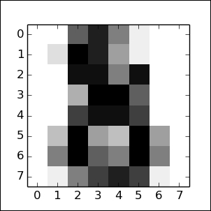
When we apply RFE over the digits dataset, we can see that it broadly captures this information in applying a ranking:
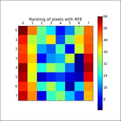
The first pixels to be cut were in and around the (typically empty) vertical edges of the image. Next, the algorithm began culling normally whitespace areas around the vertical edges or near the top of the image. The pixels that were retained longest were those that enabled the most differentiation between the different characters—pixels that would be present for some numbers and not for others.
This example gives us great visual confirmation that RFE works. What it doesn't give us is evidence for how consistently the technique works. The stability of RFE is dependent on the stability of the base model and, in some cases, ridge regression will provide a more stable solution. (For more information on which cases and the conditions involved, consult the Further reading section at the end of this chapter.)
Earlier in this chapter, we discussed the existence of algorithms that enable feature selection with very large parameter sets. Some of the most prominent techniques of this type are genetic algorithms, which emulate natural selection to generate increasingly effective models.
A genetic solution for feature selection works roughly as follows:
- An initial set of variables (predictors is the term typically used in this context) are combined into multiple subsets (candidates) and a performance measure is calculated for each candidate
- The predictors from candidates with the best performance are randomly recombined into a new iteration (generation) of models
- During this recombination step, for each subset there is the probability of a mutation, whereby a predictor may be added or removed from a subset
This algorithm typically iterates for multiple generations. The appropriate iteration amount is dependent on the complexity of the dataset and the model required. As with gradient descent techniques, the typical relationship between the performance and iteration count is present for genetic algorithms, where performance improvement declines nonlinearly as the count of iterations increases, eventually hitting a minimum before the overfitting risk increases.
To find an effective iteration count, we can perform testing using training data; by running the model for a large number of iterations and plotting the Root Mean Squared Error (RMSE), we're able to find an appropriate amount of iterations given our input data and model configuration.
Let's talk in a little more detail about what happens within each generation. Specifically, let's talk about how candidates are created, how performance is scored, and how recombination is performed.
The candidates are initially configured to use a random sample of the available predictors. There is no hard and fast rule concerning how many predictors to use in the first generation; it depends on how many features are available, but it's common to see first generation candidates using 50% to 80% of the available features (with a smaller percentage used in cases with more features).
The fitness measure can be difficult to define, but a common practice is to use two forms of cross-validation. Internal cross-validation (testing each model solely in the context of its own parameters without comparing models) is typically used to track performance at a given iteration; the fitness measures from internal cross-validation are used to select models to recombine in the next generation. External cross-validation (testing against a dataset that was not used in validation at any iteration) is also needed in order to confirm that the search process produced a model that has not overfitted to the internal training data.
Recombination is controlled by three key parameters: mutation, cross-over probabilities, and elitism. The latter is an optional parameter that one may use to reserve n-many of the top-performing models from the current generation; by doing so, one may preserve particularly effective candidates from being lost entirely during recombination. This can be done while also using that candidate in mutated variants and/or using them as parents to next-generation candidates.
The mutation probability defines the chance of a next-generation model being randomly readjusted (via some predictors, typically one, being added or removed). Mutation tends to help the genetic algorithm maintain a broad coverage of the candidate variables, reducing the risk of falling into a parameter-local solution.
Cross-over probability defines the likelihood that a pair of candidates will be selected for recombination into a next-generation model. There are several cross-over algorithms: parts of each parent's feature set might be spliced (for example, first half/second half) into the child or a random selection of each parent's features might be used. Common features to both parents might also be used by default. Random sampling from the set of both parent's unique predictors is a common default approach.
These are the main parts of a general genetic algorithm, which can be used as a wrapper to existing models (logistic regression, SVM, and others). The technique described here can be varied in many different ways and is related to feature selection techniques used slightly differently across multiple quantitative fields. Let's take the theory that we've covered thus far and start applying it to a practical example.