Vowpal Wabbit (VW) is an open source project for a fast online learner initially released in 2007 by John Langford, Lihong Li, and Alex Strehl from Yahoo! Research (http://hunch.net/?p=309) and then successively sponsored by Microsoft Research, as John Langford became the principal researcher at Microsoft. The project has developed over the years, arriving today at version 8.1.0 (at the time this chapter was written), with almost one hundred contributors working on it. (For a visualization of the development of the contributions over time, there is an interesting video using the software Gource at https://www.youtube.com/watch?v=-aXelGLMMgk.). To date, VW is still being constantly developed and keeps on increasing its learning capabilities at each development iteration.

The striking characteristic of VW is that it is very fast compared to other solutions available (LIBLINEAR, Sofia-ml, svmsgd, and Scikit-learn). Its secret is simple, yet extremely effective: it can load data and learn from it at the same time. An asynchronous thread does the parsing of the examples flowing in as a number of learning threads work on a disjoint set of features, thus assuring a high computational efficiency even when parsing involves high-dimensional feature creation (such as quadratic or cubic polynomial expansion). In most cases, the real bottleneck of the learning process is the transmission bandwidth of the disk or network transmitting the data to VW.

VW can work out classification (even multiclass and multilabel), regression (OLS and quantile), and active learning problems, offering a vast range of accompanying learning tools (called reductions) such as matrix factorization, Latent Dirichlet Allocation (LDA), neural networks, n-grams for language models, and bootstrapping.

VW can be retrieved from the online versioning repository GitHub (https://github.com/JohnLangford/vowpal_wabbit), where it can be Git-cloned or just downloaded in the form of a packed zip. Being developed on Linux systems, it is easily compiled on any POSIX environment by a simple sequence of make and make install commands. Detailed instructions for installation are available directly on its installation page and you can download Linux precompiled binaries directly from the author (https://github.com/JohnLangford/vowpal_wabbit/wiki/Download).

A VW version working on Windows operating systems, unfortunately, is a bit more difficult to obtain. In order to create one, the first reference is the documentation itself of VW where a compiling procedure is explained in detail (https://github.com/JohnLangford/vowpal_wabbit/blob/master/README.windows.txt).

VW can work with a particular data format and is invoked from a shell. John Langford uses this sample dataset for his online tutorial (https://github.com/JohnLangford/vowpal_wabbit/wiki/Tutorial), representing three houses whose roofs could be replaced. We find it interesting proposing it to you and commenting on it together:

In: 
with open('house_dataset','wb') as W:
    W.write("0 | price:.23 sqft:.25 age:.05 2006
")
    W.write("1 2 'second_house | price:.18 sqft:.15 age:.35 1976
")
    W.write("0 1 0.5 'third_house | price:.53 sqft:.32 age:.87 1924
")

with open('house_dataset','rb') as R:
    for line in R:
        print line.strip()

Out:
0 | price:.23 sqft:.25 age:.05 2006
1 2 'second_house | price:.18 sqft:.15 age:.35 1976
0 1 0.5 'third_house | price:.53 sqft:.32 age:.87 1924

The first noticeable aspect of the file format is that it doesn't have a header. This is because VW uses the hashing trick to allocate the features into a sparse vector, therefore knowing in advance the features that are not necessary at all. Data blocks are divided by pipes (the character|) into namespaces, to be intended as different clusters of features, each one containing one or more features.

The first namespace is always the one containing the response variable. The response can be a real number (or an integer) pointing out a numeric value to be regressed, a binary class, or a class among multiple ones. The response is always the first number to be found on a line. A binary class can be encoded using 1 for positive and -1 for negative (using 0 as a response is allowed only for regression). Multiple classes should be numbered from 1 onward and having gap numbers is not advisable because VW asks for the last class and considers all the integers between 1 and the last one.

The number immediately after the response value is the weight (telling you if you have to consider an example as a multiple example or as a fraction of one), then the base, which plays the role of the initial prediction (a kind of bias). Finally, preceded by the apostrophe character ('), there is the label, which can be a number or text to be later found in the VW outputs (in a prediction, you have an identifier for every estimation). Weight, base, and labels are not compulsory: if omitted, weight will be imputed as 1 and base and label won't matter.

Following the first namespace, you can add as many namespaces as you want, labeling each one by a number or string. In order to be considered the label of the namespace, it should be stuck to the pipe, for instance, |label.

After the label of the namespace, you can add any feature by its name. The feature name can be anything, but should contain a pipe or colon. You can just put entire texts in the namespaces and every word will be treated as a feature. Every feature will be considered valued as 1. If you want to assign a different number, just stick a colon at the end of the feature name and put its value after it.

For instance, a valid row readable by Vowpal Wabbit is:

0 1 0.5 'third_house | price:.53 sqft:.32 age:.87 1924

In the first namespace, the response is 0, the example weights 1, the base is 0.5, and its label is third_house. The namespace is nameless and is constituted by four features such as price (value is .53), sqft (value is .32), age (value is .87), and 1924 (value is 1).

If you have a feature in an example but not in another one, the algorithm will pretend that the feature value is zero in the second example. Therefore, a feature such as 1924 in the preceding example can be intended as a binary variable as, when it is present, it is automatically valued 1, when missing 0. This also tells you how VW handles missing values—it automatically considers them as 0 values.

There are a few packages integrating it with Python (vowpal_porpoise, Wabbit Wappa, or pyvw) and installing them is easy in Linux systems, but much harder on Windows. No matter whether you are working with Jupyter or IDE, the easiest way to use VW integrated with Python's scripts is to leverage the Popen function from the subprocess package. That makes VW run in parallel with Python. Python just waits for VW to complete its operation by capturing its output and printing it on the screen:

In: import subprocess

def execute_vw(parameters):
    execution = subprocess.Popen('vw '+parameters, 
                shell=True, stderr=subprocess.PIPE)
    line = ""
    history = ""
    while True:
        out = execution.stderr.read(1)
        history += out
        if out == '' and execution.poll() != None:
            print '------------ COMPLETED ------------
'
            break
        if out != '':
            line += out
            if '
' in line[-2:]:
                print line[:-2]
                line = ''
    return history.split('
')

The functions return a list of the outputs of the learning process, making it easy to process it, extracting relevant reusable information (like the error measure). As a precondition for its correct functioning, place the VW executable (the vw.exe file) in the Python working directory or system path where it can be found.

By invoking the function on the previously recorded housing dataset, we can have a look at how it works and what outputs it produces:

In:
params = "house_dataset"
results = execute_vw(params)

Out:
Num weight bits = 18
learning rate = 0.5
initial_t = 0
power_t = 0.5
using no cache
Reading datafile = house_dataset
num sources = 1
average  since         example        example  current  current  current
loss     last          counter         weight    label  predict features
0.000000 0.000000            1            1.0   0.0000   0.0000        5
0.666667 1.000000            2            3.0   1.0000   0.0000        5

finished run
number of examples per pass = 3
passes used = 1
weighted example sum = 4.000000
weighted label sum = 2.000000
average loss = 0.750000
best constant = 0.500000
best constant's loss = 0.250000
total feature number = 15
------------ COMPLETED ------------

The initial rows of the output just recall the used parameters and provide confirmation of which data file is being used. Most interesting is the progressive reported by the number of streamed examples (reported by the power of 2, so example 1, 2, 4, 8, 16, and so on). With respect to the loss function, an average loss measure is reported, progressive for the first iteration, based on the hold-out set afterward, whose loss is signaled by postponing the letter h (if holding out is excluded, it is possible that just the in-sample measure is reported). On the example weight column, the weight of the example is reported and then the example is furthermore described as current label, current predict and displays the number of features found on that line (current features). All such information should help you keep an eye on the stream and learning process.

After the learning is completed, a few reporting measures are reported. The average loss is the most important, in particular when a hold-out is used. Using such loss is most useful for comparative reasons as it can be immediately compared with best constant's loss (the baseline predictive power of a simple constant) and with different runs using different parameter configurations.

Another very useful function to integrate VW and Python is a function that we prepared automatically converting CSV files to VW data files. You can find it in the following code snippet. It will help us replicate the previous bike-sharing and covertype problems using VW this time, but it can be easily reused for your own projects:

In: import csv

def vw_convert(origin_file, target_file, binary_features, numeric_features, target, transform_target=lambda(x):x,
               separator=',', classification=True, multiclass=False, fieldnames= None, header=True, sparse=True):
    """
    Reads a online style stream and returns a generator of normalized feature vectors

    Parameters
----------
    original_file = the CSV file you are taken the data from 
    target file = the file to stream from
    binary_features = the list of qualitative features to consider
    numeric_features = the list of numeric features to consider
    target = the label of the response variable
    transform_target = a function transforming the response
    separator = the field separator character
    classification = a Boolean indicating if it is classification
    multiclass =  a Boolean for multiclass classification
    fieldnames = the fields' labels (can be omitted and read from file)
    header = a boolean indicating if the original file has an header
    sparse = if a sparse vector is to be returned from the generator
    """
    with open(target_file, 'wb') as W:
        with open(origin_file, 'rb') as R:
iterator = csv.DictReader(R, fieldnames, delimiter=separator)
            for n, row in enumerate(iterator):
                if not header or n>0:
                # DATA PROCESSING
                    response = transform_target(float(row[target]))
                    if classification and not multiclass:
                            if response == 0:
                                stream_row = '-1 '
                            else:
                                stream_row = '1 '
                    else:
                        stream_row = str(response)+' '
                    quantitative = list()
                    qualitative  = list()
                    for k,v in row.iteritems():
                        if k in binary_features:
                            qualitative.append(str(k)+
'_'+str(v)+':1')
                        else:
                            if k in numeric_features and (float(v)!=0 or not sparse):
                                quantitative.append(str(k)+':'+str(v))
if quantitative:
                        stream_row += '|n '+
' '.join(quantitative)
                    if qualitative:
                        stream_row += '|q '+
' '.join(qualitative)
W.write(stream_row+'
')

VW works on minimizing a general cost function, which is as follows:

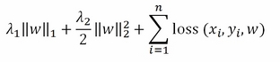
As in other formulations seen before, w is the coefficient vector and the optimization is obtained separately for each xi and yi according to the chosen loss function (OLS, logistic, or hinge). Lambda1 and lambda2 are the regularization parameters that, by default, are zero but can be set using the --l1 and --l2 options in the VW command line.

Given such a basic structure, VW has been made more complex and complete over time using the reduction paradigm. A reduction is just a way to reuse an existing algorithm in order to solve new problems without coding new solving algorithms from scratch. In other words, if you have a complex machine learning problem A, you just reduce it to B. Solving B hints at a solution of A. This is also justified by the growing interest in machine learning and the exploding number of problems that cannot be solved creating hosts of new algorithms. It is an interesting approach leveraging the existing possibilities offered by basic algorithms and the reason why VW has grown its applicability over time though the program has stayed quite compact. If you are interested in this approach, you can have a look at these two tutorials from John Langford: http://hunch.net/~reductions_tutorial/ and http://hunch.net/~jl/projects/reductions/reductions.html.

For other illustration purposes, we will briefly introduce you to a couple of reductions to implement an SVM with an RBFkernel and a shallow neural network using VW in a purely out-of-core way. We will be using some toy datasets for the purpose.

Here is the Iris dataset, changed to a binary classification problem to guess the Iris Versicolor from the Setosa and Virginica:

In: import numpy as np
from sklearn.datasets import load_iris, load_boston
from random import seed
iris = load_iris()
seed(2)
re_order = np.random.permutation(len(iris.target))
with open('iris_versicolor.vw','wb') as W1:
    for k in re_order:
        y = iris.target[k]
        X = iris.values()[1][k,:]
        features = ' |f '+' '.join([a+':'+str(b) for a,b in zip(map(lambda(a): a[:-5].replace(' ','_'), iris.feature_names),X)])
        target = '1' if y==1 else '-1'
        W1.write(target+features+'
')

Then for a regression problem, we will be using the Boston house pricing dataset:

In: boston = load_boston()
seed(2)
re_order = np.random.permutation(len(boston.target))
with open('boston.vw','wb') as W1:
     for k in re_order:
        y = boston.target[k]
        X = boston.data[k,:]
        features = ' |f '+' '.join([a+':'+str(b) for a,b in zip(map(lambda(a): a[:-5].replace(' ','_'), iris.feature_names),X)])
        W1.write(str(y)+features+'
')

First, we will be trying SVM. kvsm is a reduction based on the LaSVM algorithm (Fast Kernel Classifiers with Online and Active Learning—http://www.jmlr.org/papers/volume6/bordes05a/bordes05a.pdf) without a bias term. The VW version typically works in just one pass and with a 1-2 reprocessing of a randomly picked support vector (though some problems may need multiple passes and reprocessing). In our case, we are just using a single pass and a couple of reprocessings in order to fit an RBF kernel on our binary problem (KSVM works only for classification problems). Implemented kernels are linear, radial basis function, and polynomial. In order to have it work, use the --ksvm option, set a number for reprocessing (default is 1) by --reprocess, choose the kernel with --kernel (options are linear, poly, and rbf). Then, if the kernel is polynomial, set an integer number for --degree, or a float (default is 1.0) for --bandwidth if you are using RBF. You also have to compulsorily specify l2 regularization; otherwise, the reduction won't work properly. In our example, we make an RBFkernel with bandwidth 0.1:

In: params = '--ksvm --l2 0.000001 --reprocess 2 -b 18 --kernel rbf --bandwidth=0.1 -p iris_bin.test -d iris_versicolor.vw'
results = execute_vw(params)

accuracy = 0
with open('iris_bin.test', 'rb') as R:
    with open('iris_versicolor.vw', 'rb') as TRAIN:
        holdouts = 0.0
        for n,(line, example) in enumerate(zip(R,TRAIN)):
            if (n+1) % 10==0:
                predicted = float(line.strip())
                y = float(example.split('|')[0])
                accuracy += np.sign(predicted)==np.sign(y)
                holdouts += 1            
print 'holdout accuracy: %0.3f' % ((accuracy / holdouts)**0.5)

Out: holdout accuracy: 0.966

Neural networks are another cool addition to VW; thanks to the work of Paul Mineiro (http://www.machinedlearnings.com/2012/11/unpimp-your-sigmoid.html), VW can implement a single-layer neural network with hyperbolic tangent (tanh) activation and, optionally, dropout (using the --dropout option). Though it is only possible to decide the number of neurons, the neural reduction works fine with both regression and classification problems and can smoothly take on other transformations by VW as inputs (such as quadratic variables and n-grams), making it a very well-integrated, versatile (neural networks can solve quite a lot of problems), and fast solution. In our example, we apply it to the Boston dataset using five neurons and dropout:

In: params = 'boston.vw -f boston.model --loss_function squared -k --cache_file cache_train.vw --passes=20 --nn 5 --dropout'
results = execute_vw(params)
params = '-t boston.vw -i boston.model -k --cache_file cache_test.vw -p boston.test'
results = execute_vw(params)
val_rmse = 0
with open('boston.test', 'rb') as R:
    with open('boston.vw', 'rb') as TRAIN:
        holdouts = 0.0
        for n,(line, example) in enumerate(zip(R,TRAIN)):
            if (n+1) % 10==0:
                predicted = float(line.strip())
                y = float(example.split('|')[0])
                val_rmse += (predicted - y)**2
                holdouts += 1            
print 'holdout RMSE: %0.3f' % ((val_rmse / holdouts)**0.5)

Out: holdout RMSE: 7.010

Let's try VW on the previously created bike-sharing example file in order to explain the output components. As the first step, you have to transform the CSV file into a VW file and the previous vw_convert function will come in handy doing this. As before, we will apply a logarithmic transformation on the numeric response, using the apply_log function passed by the transform_target parameter of the vw_convert function:

In: import os
import numpy as np

def apply_log(x): 
    return np.log(x + 1.0)

def apply_exp(x): 
    return np.exp(x) - 1.0

local_path = os.getcwd()
b_vars = ['holiday','hr','mnth', 'season','weathersit','weekday','workingday','yr']
n_vars = ['hum', 'temp', 'atemp', 'windspeed']
source = '\bikesharing\hour.csv'
origin = target_file=local_path+''+source
target = target_file=local_path+''+'bike.vw'
vw_convert(origin, target, binary_features=b_vars, numeric_features=n_vars, target = 'cnt', transform_target=apply_log,
               separator=',', classification=False, multiclass=False, fieldnames= None, header=True)

After a few seconds, the new file should be ready. We can immediately run our solution, which is a simple linear regression (the default option in VW). The learning is expected to run for 100 passes, controlled by the out-of-sample validation that VW automatically implements (drawing systematically and in a repeatable way, a single observation out of every 10 as validation). In this case, we decide to set a holdout sample after 16,000 examples (using the --holdout_after option). When the validation error on the validation increases (instead of decreasing), VW stops after a few iterations (three by default, but the number can be changed using the --early_terminate option), avoiding overfitting the data:

In: params = 'bike.vw -f regression.model -k --cache_file cache_train.vw --passes=100 --hash strings --holdout_after 16000'
results = execute_vw(params)

Out: …
finished run
number of examples per pass = 15999
passes used = 6
weighted example sum = 95994.000000
weighted label sum = 439183.191893
average loss = 0.427485 h
best constant = 4.575111
total feature number = 1235898
------------ COMPLETED ------------

The final report indicates that six passes (out of 100 possible ones) have been completed and the out-of-sample average loss is 0.428. As we are interested in RMSE and RMSLE, we have to calculate them ourselves.

We then predict the results in a file (pred.test) in order to be able to read them and calculate our error measure using the same holdout strategy as in the training set. The results are indeed much better (in a fraction of the time) than what we previously obtained with Scikit-learn's SGD:

In: params = '-t bike.vw -i regression.model -k --cache_file cache_test.vw -p pred.test'
results = execute_vw(params)
val_rmse = 0
val_rmsle = 0
with open('pred.test', 'rb') as R:
    with open('bike.vw', 'rb') as TRAIN:
        holdouts = 0.0
        for n,(line, example) in enumerate(zip(R,TRAIN)):
            if n > 16000:
                predicted = float(line.strip())
                y_log = float(example.split('|')[0])
                y = apply_exp(y_log)
                val_rmse += (apply_exp(predicted) - y)**2
                val_rmsle += (predicted - y_log)**2
                holdouts += 1

print 'holdout RMSE: %0.3f' % ((val_rmse / holdouts)**0.5)
print 'holdout RMSLE: %0.3f' % ((val_rmsle / holdouts)**0.5)

Out:
holdout RMSE: 135.306
holdout RMSLE: 0.845

The covertype problem can also be solved better and more easily by VW than we managed before. This time, we will have to set some parameters and decide on the error correcting tournament (ECT, invoked by the--ect parameter on VW), where each class competes in an elimination tournament to be the label for an example. In many examples, ECT can outperform one-against-all (OAA), but this is not a general rule, and ECT is one of the approaches to be tested when dealing with multiclass problems. (The other possible option is --log_multi, using online decision trees to split the sample in smaller sets where we apply single predictive models.) We also set the learning rate to 1.0 and create a third-degree polynomial expansion using the --cubic parameter, pointing out which namespaces have to be multiplied by each other (In this case, the namespace f for three times is expressed by the nnn string followed by --cubic.):

In: import os
local_path = os.getcwd()
n_vars = ['var_'+'0'*int(j<10)+str(j) for j in range(54)]
source = 'shuffled_covtype.data'
origin = target_file=local_path+''+source
target = target_file=local_path+''+'covtype.vw'
vw_convert(origin, target, binary_features=list(), fieldnames= n_vars+['covertype'], numeric_features=n_vars,
    target = 'covertype', separator=',', classification=True, multiclass=True, header=False, sparse=False)
params = 'covtype.vw --ect 7 -f multiclass.model -k --cache_file cache_train.vw --passes=2 -l 1.0 --cubic nnn'
results = execute_vw(params)

Out:
finished run
number of examples per pass = 522911
passes used = 2
weighted example sum = 1045822.000000
weighted label sum = 0.000000
average loss = 0.235538 h
total feature number = 384838154
------------ COMPLETED ------------

Here, we wouldn't need to inspect the error measure further as the reported average loss is the complement to 1.0 of the accuracy measure; we just calculate it for completeness, confirming that our holdout accuracy is exactly 0.769:

In: params = '-t covtype.vw -i multiclass.model -k --cache_file cache_test.vw -p covertype.test'
results = execute_vw(params)
accuracy = 0
with open('covertype.test', 'rb') as R:
    with open('covtype.vw', 'rb') as TRAIN:
        holdouts = 0.0
        for n,(line, example) in enumerate(zip(R,TRAIN)):
            if (n+1) % 10==0:
                predicted = float(line.strip())
                y = float(example.split('|')[0])
                accuracy += predicted ==y
                holdouts += 1
print 'holdout accuracy: %0.3f' % (accuracy / holdouts)

Out: holdout accuracy: 0.769