
We started this chapter with bagging; now we will complete our overview with boosting, a different ensemble method. Just like bagging, boosting can be used for both regression and classification and has recently overshadowed random forest for higher accuracy.
As an optimization process, boosting is based on the stochastic gradient descent principle that we have seen in other methods, namely optimizing models by minimizing error according to gradients. The most familiar boosting methods to date are AdaBoost and Gradient Boosting (GBM and recently XGBoost). The AdaBoost algorithm comes down to minimizing the error of those cases where the prediction is slightly wrong so that cases that are harder to classify get more attention. Recently, AdaBoost fell out of favor as other boosting methods were found to be generally more accurate.
In this chapter, we will cover the two most effective boosting algorithms available to date to Python users: Gradient Boosting Machine (GBM) found in the Scikit-learn package and extreme gradient boosting (XGBoost). As GBM is sequential in nature, the algorithm is hard to parallelize and thus harder to scale than random forest, but some tricks will do the job. Some tips and tricks to speed up the algorithm will be covered with a nice out-of-memory solution for H2O.
As we have seen in the previous sections, random forests and extreme trees are efficient algorithms and both work quite well with minimum effort. Though recognized as a more accurate method, GBM is not very easy to use and it is always necessary to tune its many hyperparameters in order to achieve the best results. Random forest, on the other hand, can perform quite well with only a few parameters to consider (mostly tree depth and number of trees). Another thing to pay attention to is overtraining. Random forests are less sensitive to overtraining than GBM. So, with GBM, we also need to think about regularization strategies. Above all, random forests are much easier to perform parallel operations where as GBM is sequential and thus slower to compute.
In this chapter, we will apply GBM in Scikit-learn, look at the next generation of tree boosting algorithms named XGBoost, and implement boosting on a larger scale on H2O.
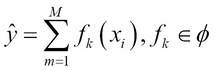
The GBM algorithm that we use in Scikit-learn and H2O is based on two important concepts: additive expansion and gradient optimization by the steepest descent algorithm. The general idea of the former is to generate a sequence of relatively simple trees (weak learners), where each successive tree is added along a gradient. Let's assume that we have M trees that aggregate the final predictions in the ensemble. The tree in each iteration fk is now part of a much broader space of all the possible trees in the model (![]() ) (in Scikit-learn, this parameter is better known as
) (in Scikit-learn, this parameter is better known as n_estimators):
The additive expansion will add new trees to previous trees in a stage-wise manner:
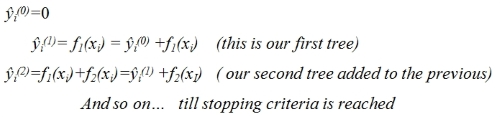
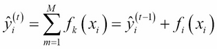
The prediction of our gradient boosting ensemble is simply the sum of the predictions of all the previous trees and the newly added tree ![]() , more formally leading to the following:
, more formally leading to the following:
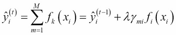
The second important and yet quite tricky part of the GBM algorithm is gradient optimization by steepest descent. This means that we add increasingly more powerful trees to the additive model. This is achieved by applying gradient optimization to the new trees. How do we perform gradient updates with trees as there are no parameters like we have seen with traditional learning algorithms? First, we parameterize the trees; we do this by recursively upgrading the node split values along a gradient where the nodes are represented by a vector. This way, the steepest descent direction is the negative gradient of the loss function and the node splits will be upgraded and learned, leading to:
 : A shrinkage parameter (also referred to as learning rate in this context) that will cause the ensemble to learn slowly with the addition of more trees
 : The gradient upgrade parameter also referred to as the step length
The prediction score for each leaf is thus the final score for the new tree that then simply is the sum over each leaf:
So to summarize, GBM works by incrementally adding more accurate trees learned along the gradient.
Now that we understand the core concepts, let's run a GBM example and look at the most important parameters. For GBM, these parameters are extra important because when we set this number of trees too high, we are bound to strain our computational resources exponentially. So be careful with these parameters. Most parameters in Scikit-learn's GBM application are the same as in random forest, which we have covered in the previous paragraph. There are three parameters that we need to take into account that need special attention.
Contrary to random forests, which perform better when they build their tree structures to their maximum extension (thus building and ensembling predictors with high variance), GBM tends to work better with smaller trees (thus leveraging predictors with a higher bias, that is, weak learners). Working with smaller decision trees or just with stumps (decision trees with only one single branch) can alleviate the training time, trading off the speediness of execution against a larger bias (because a smaller tree can hardly intercept more complex relationships in data).
Also known as shrinkage ![]() , this is a parameter related to the gradient descent optimization and how each tree will contribute to the ensemble. Smaller values of this parameter can improve the optimization in the training process, though it will require more estimators to converge and thus more computational time. As it affects the weight of each tree in the ensemble, smaller values imply that each tree will contribute a small part to the optimization process and you will need more trees before reaching a good solution. Consequently, when optimizing this parameter for performance, we should avoid too large values that may lead to sub-optimal models; we also have to avoid using too low values because this will affect the computation time heavily (more trees will be needed for the ensemble to converge to a solution). In our experience, a good starting point is to use a learning rate in the range <0.1 and >.001.
, this is a parameter related to the gradient descent optimization and how each tree will contribute to the ensemble. Smaller values of this parameter can improve the optimization in the training process, though it will require more estimators to converge and thus more computational time. As it affects the weight of each tree in the ensemble, smaller values imply that each tree will contribute a small part to the optimization process and you will need more trees before reaching a good solution. Consequently, when optimizing this parameter for performance, we should avoid too large values that may lead to sub-optimal models; we also have to avoid using too low values because this will affect the computation time heavily (more trees will be needed for the ensemble to converge to a solution). In our experience, a good starting point is to use a learning rate in the range <0.1 and >.001.
Let's recall the principles of bagging and pasting, where we take random samples and construct trees on those samples. If we apply subsampling to GBM, we randomize the tree constructions and prevent overfitting, reduce memory load, and even sometimes increase accuracy. We can apply this procedure to GBM as well, making it more stochastic and thus leveraging the advantages of bagging. We can randomize the tree construction in GBM by setting the subsample parameter to .5.
This parameter allows storing new tree information after each iteration is added to the previous one without generating new trees. This way, we can save memory and speed up computation time extensively.
Using the GBM available in Scikit-learn, there are two actions that we can take in order to increase memory and CPU efficiency:
- Warm start for (semi) incremental learning
- We can use parallel processing during cross-validation
Let's run through a GBM classification example where we use the spam dataset from the UCI machine learning library. We will first load the data, preprocess it, and look at the variable importance of each feature:
import pandas
import urllib2
import urllib2
from sklearn import ensemble
columnNames1_url = 'https://archive.ics.uci.edu/ml/machine-learning-databases/spambase/spambase.names'
columnNames1 = [
   line.strip().split(':')[0]
   for line in urllib2.urlopen(columnNames1_url).readlines()[33:]]

columnNames1
n = 0
for i in columnNames1:
   columnNames1[n] = i.replace('word_freq_','')
   n += 1
print columnNames1

spamdata = pandas.read_csv(
   'https://archive.ics.uci.edu/ml/machine-learning-databases/spambase/spambase.data',
   header=None, names=(columnNames1 + ['spam'])
)

X = spamdata.values[:,:57]
y=spamdata['spam']

spamdata.head()

import numpy as np
from sklearn import cross_validation
from sklearn.metrics import classification_report
from sklearn.cross_validation import cross_val_score
from sklearn.cross_validation import cross_val_predict
from sklearn.cross_validation import train_test_split
from sklearn.metrics  import recall_score, f1_score
from sklearn.cross_validation import cross_val_predict
import matplotlib.pyplot as plt
from sklearn.metrics import confusion_matrix
from sklearn.metrics import accuracy_score
from sklearn.ensemble import GradientBoostingClassifier

X_train, X_test, y_train, y_test = train_test_split(X,y, test_size=0.3, random_state=22)

clf = ensemble.GradientBoostingClassifier(n_estimators=300,random_state=222,max_depth=16,learning_rate=.1,subsample=.5)
scores=clf.fit(X_train,y_train)
scores2 = cross_val_score(clf, X_train, y_train, cv=3, scoring='accuracy',n_jobs=-1)
print scores2.mean()

y_pred = cross_val_predict(clf, X_test, y_test, cv=10)
print 'validation accuracy %s' % accuracy_score(y_test, y_pred)

OUTPUT:]
validation accuracy 0.928312816799

confusionMatrix = confusion_matrix(y_test, y_pred)
print confusionMatrix

from sklearn.metrics import accuracy_score
accuracy_score(y_test, y_pred)

clf.feature_importances_

def featureImp_order(clf, X, k=5):
    return X[:,clf.feature_importances_.argsort()[::-1][:k]]
newX = featureImp_order(clf,X,2)
print newX

# let's order the features in amount of importance

print sorted(zip(map(lambda x: round(x, 4), clf.feature_importances_), columnNames1),
    reverse=True)
OUTPUT]

0.945030177548
    precision    recall  f1-score   support

    0       0.93      0.96      0.94       835
    1       0.93      0.88      0.91       546

avg / total       0.93      0.93      0.93      1381

[[799  36]
 [ 63 483]]


Feature importance:

[(0.2262, 'char_freq_;'),
(0.0945, 'report'),
(0.0637, 'capital_run_length_average'),
(0.0467, 'you'),
(0.0461, 'capital_run_length_total')
(0.0403, 'business')
(0.0397, 'char_freq_!')
(0.0333, 'will')
(0.0295, 'capital_run_length_longest')
(0.0275, 'your')
(0.0259, '000')
(0.0257, 'char_freq_(')
(0.0235, 'char_freq_$')
(0.0207, 'internet')
We can see that the character ; is the most discriminative in classifying spam.
Unfortunately, there is no parallel processing for GBM in Scikit-learn. Only cross-validation and gridsearch can be parallelized. So what can we do to make it faster? We saw that GBM works with the principle of additive expansion where trees are added incrementally. We can utilize this idea in Scikit-learn with the warm-start parameter. We can model this with Scikit-learn's GBM functionalities by building tree models incrementally with a handy for loop. So let's do this with the same dataset and inspect the computational advantage that it provides:
gbc = GradientBoostingClassifier(warm_start=True, learning_rate=.05, max_depth=20,random_state=0)
for n_estimators in range(1, 1500, 100):
    gbc.set_params(n_estimators=n_estimators)
    gbc.fit(X_train, y_train)
y_pred = gbc.predict(X_test)
print(classification_report(y_test, y_pred))
print(gbc.set_params)
OUTPUT:
 precision    recall  f1-score   support

    0       0.93      0.95      0.94       835
    1       0.92      0.89      0.91       546

avg / total       0.93      0.93      0.93      1381

<bound method GradientBoostingClassifier.set_params of GradientBoostingClassifier(init=None, learning_rate=0.05, loss='deviance',
    max_depth=20, max_features=None, max_leaf_nodes=None,
    min_samples_leaf=1, min_samples_split=2,
    min_weight_fraction_leaf=0.0, n_estimators=1401,
    presort='auto', random_state=0, subsample=1.0, verbose=0,
    warm_start=True)>
It's adviable to pay special attention to the output of the settings of the tree (n_estimators=1401). You can see that the size of the tree we used is 1401. This little trick helped us reduce the training time a lot (think half or even less) when we compare it to a similar GBM model, which we would have trained with 1401 trees at once. Note that we can use this method for random forest and extreme random forest as well. Nevertheless, we found this useful specifically for GBM.
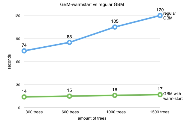
Let's look at the figure that shows the training time for a regular GBM and our warm_start method. The computation speedup is considerable with the accuracy remaining relatively the same:
Ever thought of training a model on three computers at the same time? Or training a GBM model on an EC2 instance? There might be a case where you train a model and want to store it to use it again later on. When you have to wait for two days for a full training round to complete, we don't want to have to go through that process again. A case where you have trained a model in the cloud on an Amazon EC2 instance, you can store that model and reuse it later on another computer using Scikit-learn's joblib. So let's walk through this process as Scikit-learn has provided us with a handy tool to manage it.
Let's import the right libraries and set our directories for our file locations:
import errno
import os
#set your path here
path='/yourpath/clfs'
clfm=os.makedirs(path)
os.chdir(path)
Now let's export the model to the specified location on our harddrive:
from sklearn.externals import joblib
joblib.dump( gbc,'clf_gbc.pkl')
Now we can load the model and reuse it for other purposes:
model_clone = joblib.load('clf_gbc.pkl')
zpred=model_clone.predict(X_test)
print zpred