Let's implement a random forest with gridsearch hyperparameter optimization. In this section, we first load the spam dataset from the URL source:

import pandas as pd
import numpy as np
import os
import xlrd
import urllib
import h2o

#set your path here
os.chdir('/yourpath/')

url = 'https://archive.ics.uci.edu/ml/machine-learning-databases/spambase/spambase.data'
filename='spamdata.data'
urllib.urlretrieve(url, filename)

Now that we have loaded the data, we can initialize the H2O session:

h2o.init(max_mem_size_GB = 2)

OUTPUT:

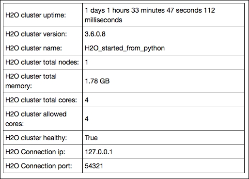
Here, we preprocess the data where we split the data into train, validation, and test sets. We do this with an H2O function (.split_frame). Also note the important step where we convert the target vector C58 to a factor variable:

spamdata = h2o.import_file(os.path.realpath("/yourpath/"))
spamdata['C58']=spamdata['C58'].asfactor()
train, valid, test= spamdata.split_frame([0.6,.2], seed=1234)
spam_X = spamdata.col_names[:-1]    
spam_Y = spamdata.col_names[-1]

In this part, we will set up the parameters that we will optimize with gridsearch. First of all, we set the number of trees in the model to a single value of 300. The parameters that are iterated with gridsearch are as follows:

Now let's pass these parameters into a Python list to be used in our H2O gridsearch model:

hyper_parameters={'ntrees':[300], 'max_depth':[3,6,10,12,50],'balance_classes':['True','False'],'sample_rate':[.5,.6,.8,.9]}
grid_search = H2OGridSearch(H2ORandomForestEstimator, hyper_params=hyper_parameters)
grid_search.train(x=spam_X, y=spam_Y,training_frame=train)
print 'this is the optimum solution for hyper parameters search %s' % grid_search.show()
OUTPUT: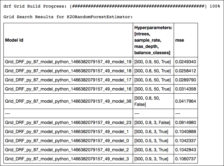

Of all the possible combinations, the model with a row sample rate of .9, a tree depth of 50, and balanced classes yields the highest accuracy. Now let's train a new random forest model with optimal parameters resulting from our gridsearch and predict the outcome on the test set:

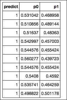
final = H2ORandomForestEstimator(ntrees=300, max_depth=50,balance_classes=True,sample_rate=.9)
final.train(x=spam_X, y=spam_Y,training_frame=train)
print final.predict(test)

The final output of the predictions in H2O results in an array with the first column containing the actual predicted classes and columns containing the class probabilities of each target label:

OUTPUT:

We have seen in previous examples that most of the time, a well-tuned GBM model outperforms random forest. So now let's perform a GBM with gridsearch in H2O and see if we can improve our score. For this session, we introduce the same random subsampling method that we used for the random forest model in H2O (sample_rate). Based on Jerome Friedman's article (https://statweb.stanford.edu/~jhf/ftp/stobst.pdf) from 1999, a method named stochastic gradient boosting was introduced. This stochasticity added to the model utilizes random subsampling without replacement from the data at each tree iteration that is considered to prevent overfitting and increase overall accuracy. In this example, we take this idea of stochasticity further by introducing random subsampling based on the features at each iteration.

This method of randomly subsampling features is also referred to as the random subspace method, which we have already seen in the Random forest and extremely randomized forest section of this chapter. We achieve this with the col_sample_rate parameter. So to summarize, in this GBM model, we are going to perform gridsearch optimization on the following parameters:

We use exactly the same spam dataset as the previous section so we can get right down to it:

hyper_parameters={'ntrees':[300],'max_depth':[12,30,50],'sample_rate':[.5,.7,1],'col_sample_rate':[.9,1],
'learn_rate':[.01,.1,.3],}
grid_search = H2OGridSearch(H2OGradientBoostingEstimator, hyper_params=hyper_parameters)
grid_search.train(x=spam_X, y=spam_Y, training_frame=train)
print 'this is the optimum solution for hyper parameters search %s' % grid_search.show()

gbm Grid Build Progress: [##################################################] 100%

The upper part of our gridsearch output shows that we should use an exceptionally high learning rate of .3, a column sample rate of .9, and a maximum tree depth of 30. Random subsampling based on rows didn't increase performance, but subsampling based on features with a fraction of .9 was quite effective in this case. Now let's train a new GBM model with the optimal parameters resulting from our gridsearch optimization and predict the outcome on the test set:

spam_gbm2 = H2OGradientBoostingEstimator(
  ntrees=300,
  learn_rate=0.3,
  max_depth=30,
  sample_rate=1,
  col_sample_rate=0.9,
  score_each_iteration=True,
  seed=2000000
)
spam_gbm2.train(spam_X, spam_Y, training_frame=train, validation_frame=valid)

confusion_matrix = spam_gbm2.confusion_matrix(metrics="accuracy")
print confusion_matrix
OUTPUT:

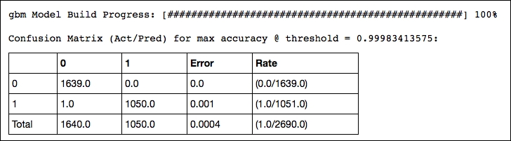
This delivers interesting diagnostics of the model's performance such as accuracy, rmse, logloss, and AUC. However, its output is too large to include here. Look at the output of your IPython notebook for the complete output.

You can utilize this with the following:

print spam_gbm2.score_history()

Of course, the final predictions can be achieved as follows:

print spam_gbm2.predict(test)

Great, we have been able to improve the accuracy of our model close to 100%. As you can see, in H2O, you might be less flexible in terms of modeling and munging your data, but the speed of processing and accuracy that can be achieved is unrivaled. To round off this session, you can do the following:

h2o.shutdown(prompt=False)