
3.2 Data Cleaning
Real-world data tend to be incomplete, noisy, and inconsistent. Data cleaning (or data cleansing) routines attempt to fill in missing values, smooth out noise while identifying outliers, and correct inconsistencies in the data. In this section, you will study basic methods for data cleaning. Section 3.2.1 looks at ways of handling missing values. Section 3.2.2 explains data smoothing techniques. Section 3.2.3 discusses approaches to data cleaning as a process.
3.2.1 Missing Values
Imagine that you need to analyze AllElectronics sales and customer data. You note that many tuples have no recorded value for several attributes such as customer income. How can you go about filling in the missing values for this attribute? Let’s look at the following methods.
1. Ignore the tuple: This is usually done when the class label is missing (assuming the mining task involves classification). This method is not very effective, unless the tuple contains several attributes with missing values. It is especially poor when the percentage of missing values per attribute varies considerably. By ignoring the tuple, we do not make use of the remaining attributes’ values in the tuple. Such data could have been useful to the task at hand.
2. Fill in the missing value manually: In general, this approach is time consuming and may not be feasible given a large data set with many missing values.
3. Use a global constant to fill in the missing value: Replace all missing attribute values by the same constant such as a label like “Unknown” or −∞. If missing values are replaced by, say, “Unknown,” then the mining program may mistakenly think that they form an interesting concept, since they all have a value in common—that of “Unknown.” Hence, although this method is simple, it is not foolproof.
4. Use a measure of central tendency for the attribute (e.g., the mean or median) to fill in the missing value: Chapter 2 discussed measures of central tendency, which indicate the “middle” value of a data distribution. For normal (symmetric) data distributions, the mean can be used, while skewed data distribution should employ the median (Section 2.2). For example, suppose that the data distribution regarding the income of AllElectronics customers is symmetric and that the mean income is $56,000. Use this value to replace the missing value for income.
5. Use the attribute mean or median for all samples belonging to the same class as the given tuple: For example, if classifying customers according to credit_risk, we may replace the missing value with the mean income value for customers in the same credit risk category as that of the given tuple. If the data distribution for a given class is skewed, the median value is a better choice.
6. Use the most probable value to fill in the missing value: This may be determined with regression, inference-based tools using a Bayesian formalism, or decision tree induction. For example, using the other customer attributes in your data set, you may construct a decision tree to predict the missing values for income. Decision trees and Bayesian inference are described in detail in Chapters 8 and 9, respectively, while regression is introduced in Section 3.4.5.
Methods 3 through 6 bias the data—the filled-in value may not be correct. Method 6, however, is a popular strategy. In comparison to the other methods, it uses the most information from the present data to predict missing values. By considering the other attributes’ values in its estimation of the missing value for income, there is a greater chance that the relationships between income and the other attributes are preserved.
It is important to note that, in some cases, a missing value may not imply an error in the data! For example, when applying for a credit card, candidates may be asked to supply their driver’s license number. Candidates who do not have a driver’s license may naturally leave this field blank. Forms should allow respondents to specify values such as “not applicable.” Software routines may also be used to uncover other null values (e.g., “don’t know,” ”?” or “none”). Ideally, each attribute should have one or more rules regarding the null condition. The rules may specify whether or not nulls are allowed and/or how such values should be handled or transformed. Fields may also be intentionally left blank if they are to be provided in a later step of the business process. Hence, although we can try our best to clean the data after it is seized, good database and data entry procedure design should help minimize the number of missing values or errors in the first place.
3.2.2 Noisy Data
“What is noise?” Noise is a random error or variance in a measured variable. In Chapter 2, we saw how some basic statistical description techniques (e.g., boxplots and scatter plots), and methods of data visualization can be used to identify outliers, which may represent noise. Given a numeric attribute such as, say, price, how can we “smooth” out the data to remove the noise? Let’s look at the following data smoothing techniques.
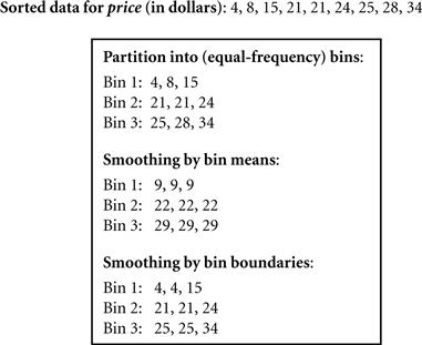
Binning: Binning methods smooth a sorted data value by consulting its “neighborhood,” that is, the values around it. The sorted values are distributed into a number of “buckets,” or bins. Because binning methods consult the neighborhood of values, they perform local smoothing. Figure 3.2 illustrates some binning techniques. In this example, the data for price are first sorted and then partitioned into equal-frequency bins of size 3 (i.e., each bin contains three values). In smoothing by bin means, each value in a bin is replaced by the mean value of the bin. For example, the mean of the values 4, 8, and 15 in Bin 1 is 9. Therefore, each original value in this bin is replaced by the value 9.
Similarly, smoothing by bin medians can be employed, in which each bin value is replaced by the bin median. In smoothing by bin boundaries, the minimum and maximum values in a given bin are identified as the bin boundaries. Each bin value is then replaced by the closest boundary value. In general, the larger the width, the greater the effect of the smoothing. Alternatively, bins may be equal width, where the interval range of values in each bin is constant. Binning is also used as a discretization technique and is further discussed in Section 3.5.
Regression: Linear regression involves finding the “best” line to fit two attributes (or variables) so that one attribute can be used to predict the other. Multiple linear regression is an extension of linear regression, where more than two attributes are involved and the data are fit to a multidimensional surface. Regression is further described in Section 3.4.5.
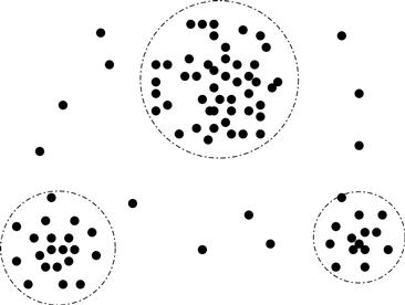
Outlier analysis: Outliers may be detected by clustering, for example, where similar values are organized into groups, or “clusters.” Intuitively, values that fall outside of the set of clusters may be considered outliers (Figure 3.3). Chapter 12 is dedicated to the topic of outlier analysis.
Many data smoothing methods are also used for data discretization (a form of data transformation) and data reduction. For example, the binning techniques described before reduce the number of distinct values per attribute. This acts as a form of data reduction for logic-based data mining methods, such as decision tree induction, which repeatedly makes value comparisons on sorted data. Concept hierarchies are a form of data discretization that can also be used for data smoothing. A concept hierarchy for price, for example, may map real price values into inexpensive, moderately_priced, and expensive, thereby reducing the number of data values to be handled by the mining process. Data discretization is discussed in Section 3.5. Some methods of classification (e.g., neural networks) have built-in data smoothing mechanisms. Classification is the topic of Chapters 8 and 9.
3.2.3 Data Cleaning as a Process
Missing values, noise, and inconsistencies contribute to inaccurate data. So far, we have looked at techniques for handling missing data and for smoothing data. “But data cleaning is a big job. What about data cleaning as a process? How exactly does one proceed in tackling this task? Are there any tools out there to help?”
The first step in data cleaning as a process is discrepancy detection. Discrepancies can be caused by several factors, including poorly designed data entry forms that have many optional fields, human error in data entry, deliberate errors (e.g., respondents not wanting to divulge information about themselves), and data decay (e.g., outdated addresses). Discrepancies may also arise from inconsistent data representations and inconsistent use of codes. Other sources of discrepancies include errors in instrumentation devices that record data and system errors. Errors can also occur when the data are (inadequately) used for purposes other than originally intended. There may also be inconsistencies due to data integration (e.g., where a given attribute can have different names in different databases).2
“So, how can we proceed with discrepancy detection?” As a starting point, use any knowledge you may already have regarding properties of the data. Such knowledge or “data about data” is referred to as metadata. This is where we can make use of the knowledge we gained about our data in Chapter 2. For example, what are the data type and domain of each attribute? What are the acceptable values for each attribute? The basic statistical data descriptions discussed in Section 2.2 are useful here to grasp data trends and identify anomalies. For example, find the mean, median, and mode values. Are the data symmetric or skewed? What is the range of values? Do all values fall within the expected range? What is the standard deviation of each attribute? Values that are more than two standard deviations away from the mean for a given attribute may be flagged as potential outliers. Are there any known dependencies between attributes? In this step, you may write your own scripts and/or use some of the tools that we discuss further later. From this, you may find noise, outliers, and unusual values that need investigation.
As a data analyst, you should be on the lookout for the inconsistent use of codes and any inconsistent data representations (e.g., “2010/12/25” and “25/12/2010” for date). Field overloading is another error source that typically results when developers squeeze new attribute definitions into unused (bit) portions of already defined attributes (e.g., an unused bit of an attribute that has a value range that uses only, say, 31 out of 32 bits).
The data should also be examined regarding unique rules, consecutive rules, and null rules. A unique rule says that each value of the given attribute must be different from all other values for that attribute. A consecutive rule says that there can be no missing values between the lowest and highest values for the attribute, and that all values must also be unique (e.g., as in check numbers). A null rule specifies the use of blanks, question marks, special characters, or other strings that may indicate the null condition (e.g., where a value for a given attribute is not available), and how such values should be handled. As mentioned in Section 3.2.1, reasons for missing values may include (1) the person originally asked to provide a value for the attribute refuses and/or finds that the information requested is not applicable (e.g., a license_number attribute left blank by nondrivers); (2) the data entry person does not know the correct value; or (3) the value is to be provided by a later step of the process. The null rule should specify how to record the null condition, for example, such as to store zero for numeric attributes, a blank for character attributes, or any other conventions that may be in use (e.g., entries like “don’t know” or ”?” should be transformed to blank).
There are a number of different commercial tools that can aid in the discrepancy detection step. Data scrubbing tools use simple domain knowledge (e.g., knowledge of postal addresses and spell-checking) to detect errors and make corrections in the data. These tools rely on parsing and fuzzy matching techniques when cleaning data from multiple sources. Data auditing tools find discrepancies by analyzing the data to discover rules and relationships, and detecting data that violate such conditions. They are variants of data mining tools. For example, they may employ statistical analysis to find correlations, or clustering to identify outliers. They may also use the basic statistical data descriptions presented in Section 2.2.
Some data inconsistencies may be corrected manually using external references. For example, errors made at data entry may be corrected by performing a paper trace. Most errors, however, will require data transformations. That is, once we find discrepancies, we typically need to define and apply (a series of) transformations to correct them.
Commercial tools can assist in the data transformation step. Data migration tools allow simple transformations to be specified such as to replace the string “gender” by “sex.” ETL (extraction/transformation/loading) tools allow users to specify transforms through a graphical user interface (GUI). These tools typically support only a restricted set of transforms so that, often, we may also choose to write custom scripts for this step of the data cleaning process.
The two-step process of discrepancy detection and data transformation (to correct discrepancies) iterates. This process, however, is error-prone and time consuming. Some transformations may introduce more discrepancies. Some nested discrepancies may only be detected after others have been fixed. For example, a typo such as “20010” in a year field may only surface once all date values have been converted to a uniform format. Transformations are often done as a batch process while the user waits without feedback. Only after the transformation is complete can the user go back and check that no new anomalies have been mistakenly created. Typically, numerous iterations are required before the user is satisfied. Any tuples that cannot be automatically handled by a given transformation are typically written to a file without any explanation regarding the reasoning behind their failure. As a result, the entire data cleaning process also suffers from a lack of interactivity.
New approaches to data cleaning emphasize increased interactivity. Potter’s Wheel, for example, is a publicly available data cleaning tool that integrates discrepancy detection and transformation. Users gradually build a series of transformations by composing and debugging individual transformations, one step at a time, on a spreadsheet-like interface. The transformations can be specified graphically or by providing examples. Results are shown immediately on the records that are visible on the screen. The user can choose to undo the transformations, so that transformations that introduced additional errors can be “erased.” The tool automatically performs discrepancy checking in the background on the latest transformed view of the data. Users can gradually develop and refine transformations as discrepancies are found, leading to more effective and efficient data cleaning.
Another approach to increased interactivity in data cleaning is the development of declarative languages for the specification of data transformation operators. Such work focuses on defining powerful extensions to SQL and algorithms that enable users to express data cleaning specifications efficiently.
As we discover more about the data, it is important to keep updating the metadata to reflect this knowledge. This will help speed up data cleaning on future versions of the same data store.