
10.4 Density-Based Methods
Partitioning and hierarchical methods are designed to find spherical-shaped clusters. They have difficulty finding clusters of arbitrary shape such as the “S” shape and oval clusters in Figure 10.13. Given such data, they would likely inaccurately identify convex regions, where noise or outliers are included in the clusters.

To find clusters of arbitrary shape, alternatively, we can model clusters as dense regions in the data space, separated by sparse regions. This is the main strategy behind density-based clustering methods, which can discover clusters of nonspherical shape. In this section, you will learn the basic techniques of density-based clustering by studying three representative methods, namely, DBSCAN (Section 10.4.1), OPTICS (Section 10.4.2), and DENCLUE (Section 10.4.3).
10.4.1 DBSCAN: Density-Based Clustering Based on Connected Regions with High Density
“How can we find dense regions in density-based clustering?” The density of an object o can be measured by the number of objects close to o. DBSCAN (Density-Based Spatial Clustering of Applications with Noise) finds core objects, that is, objects that have dense neighborhoods. It connects core objects and their neighborhoods to form dense regions as clusters.
“How does DBSCAN quantify the neighborhood of an object?” A user-specified parameter ![]() > 0 is used to specify the radius of a neighborhood we consider for every object. The
> 0 is used to specify the radius of a neighborhood we consider for every object. The ![]() -neighborhood of an object o is the space within a radius
-neighborhood of an object o is the space within a radius ![]() centered at o.
centered at o.
Due to the fixed neighborhood size parameterized by ![]() , the density of a neighborhood can be measured simply by the number of objects in the neighborhood. To determine whether a neighborhood is dense or not, DBSCAN uses another user-specified parameter, MinPts, which specifies the density threshold of dense regions. An object is a core object if the
, the density of a neighborhood can be measured simply by the number of objects in the neighborhood. To determine whether a neighborhood is dense or not, DBSCAN uses another user-specified parameter, MinPts, which specifies the density threshold of dense regions. An object is a core object if the ![]() -neighborhood of the object contains at least MinPts objects. Core objects are the pillars of dense regions.
-neighborhood of the object contains at least MinPts objects. Core objects are the pillars of dense regions.
Given a set, D, of objects, we can identify all core objects with respect to the given parameters, ![]() and MinPts. The clustering task is therein reduced to using core objects and their neighborhoods to form dense regions, where the dense regions are clusters. For a core object q and an object p, we say that p is directly density-reachable from q (with respect to
and MinPts. The clustering task is therein reduced to using core objects and their neighborhoods to form dense regions, where the dense regions are clusters. For a core object q and an object p, we say that p is directly density-reachable from q (with respect to ![]() and MinPts) if p is within the
and MinPts) if p is within the ![]() -neighborhood of q. Clearly, an object p is directly density-reachable from another object q if and only if q is a core object and p is in the
-neighborhood of q. Clearly, an object p is directly density-reachable from another object q if and only if q is a core object and p is in the ![]() -neighborhood of q. Using the directly density-reachable relation, a core object can “bring” all objects from its
-neighborhood of q. Using the directly density-reachable relation, a core object can “bring” all objects from its ![]() -neighborhood into a dense region.
-neighborhood into a dense region.
“How can we assemble a large dense region using small dense regions centered by core objects?” In DBSCAN, p is density-reachable from q (with respect to ![]() and MinPts in D) if there is a chain of objects p1, …, pn, such that p1 = q, pn = p, and pi + 1 is directly density-reachable from pi with respect to
and MinPts in D) if there is a chain of objects p1, …, pn, such that p1 = q, pn = p, and pi + 1 is directly density-reachable from pi with respect to ![]() and MinPts, for 1 ≤ i ≤ n, pi ∈ D. Note that density-reachability is not an equivalence relation because it is not symmetric. If both o1 and o2 are core objects and o1 is density-reachable from o2, then o2 is density-reachable from o1. However, if o2 is a core object but o1 is not, then o1 may be density-reachable from o2, but not vice versa.
and MinPts, for 1 ≤ i ≤ n, pi ∈ D. Note that density-reachability is not an equivalence relation because it is not symmetric. If both o1 and o2 are core objects and o1 is density-reachable from o2, then o2 is density-reachable from o1. However, if o2 is a core object but o1 is not, then o1 may be density-reachable from o2, but not vice versa.
To connect core objects as well as their neighbors in a dense region, DBSCAN uses the notion of density-connectedness. Two objects p1, p2 ∈ D are density-connected with respect to ![]() and MinPts if there is an object q ∈ D such that both p1 and p2 are density-reachable from q with respect to
and MinPts if there is an object q ∈ D such that both p1 and p2 are density-reachable from q with respect to ![]() and MinPts. Unlike density-reachability, density-connectedness is an equivalence relation. It is easy to show that, for objects o1, o2, and o3, if o1 and o2 are density-connected, and o2 and o3 are density-connected, then so are o1 and o3.
and MinPts. Unlike density-reachability, density-connectedness is an equivalence relation. It is easy to show that, for objects o1, o2, and o3, if o1 and o2 are density-connected, and o2 and o3 are density-connected, then so are o1 and o3.
Example 10.7
Density-reachability and density-connectivity
Consider Figure 10.14 for a given ![]() represented by the radius of the circles, and, say, let MinPts = 3.
represented by the radius of the circles, and, say, let MinPts = 3.
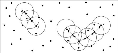
Figure 10.14 Density-reachability and density-connectivity in density-based clustering. Source: Based on Ester, Kriegel, Sander, and Xu [EKSX96].
Of the labeled points, m, p, o, r are core objects because each is in an ![]() -neighborhood containing at least three points. Object q is directly density-reachable from m. Object m is directly density-reachable from p and vice versa.
-neighborhood containing at least three points. Object q is directly density-reachable from m. Object m is directly density-reachable from p and vice versa.
Object q is (indirectly) density-reachable from p because q is directly density-reachable from m and m is directly density-reachable from p. However, p is not density-reachable from q because q is not a core object. Similarly, r and s are density-reachable from o and o is density-reachable from r. Thus, o, r, and s are all density-connected.
We can use the closure of density-connectedness to find connected dense regions as clusters. Each closed set is a density-based cluster. A subset C ⊆ D is a cluster if (1) for any two objects o1, o2 ∈ C, o1 and o2 are density-connected; and (2) there does not exist an object o ∈ C and another object o′ ∈ (D − C) such that o and o′ are density-connected.
“How does DBSCAN find clusters?” Initially, all objects in a given data set D are marked as “unvisited.” DBSCAN randomly selects an unvisited object p, marks p as “visited,” and checks whether the ![]() -neighborhood of p contains at least MinPts objects. If not, p is marked as a noise point. Otherwise, a new cluster C is created for p, and all the objects in the
-neighborhood of p contains at least MinPts objects. If not, p is marked as a noise point. Otherwise, a new cluster C is created for p, and all the objects in the ![]() -neighborhood of p are added to a candidate set, N. DBSCAN iteratively adds to C those objects in N that do not belong to any cluster. In this process, for an object p′ in N that carries the label “unvisited,” DBSCAN marks it as “visited” and checks its
-neighborhood of p are added to a candidate set, N. DBSCAN iteratively adds to C those objects in N that do not belong to any cluster. In this process, for an object p′ in N that carries the label “unvisited,” DBSCAN marks it as “visited” and checks its ![]() -neighborhood. If the
-neighborhood. If the ![]() -neighborhood of p′ has at least MinPts objects, those objects in the
-neighborhood of p′ has at least MinPts objects, those objects in the ![]() -neighborhood of p′ are added to N. DBSCAN continues adding objects to C until C can no longer be expanded, that is, N is empty. At this time, cluster C is completed, and thus is output.
-neighborhood of p′ are added to N. DBSCAN continues adding objects to C until C can no longer be expanded, that is, N is empty. At this time, cluster C is completed, and thus is output.
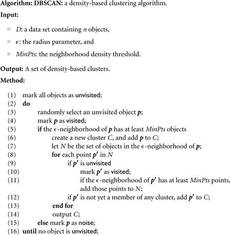
To find the next cluster, DBSCAN randomly selects an unvisited object from the remaining ones. The clustering process continues until all objects are visited. The pseudocode of the DBSCAN algorithm is given in Figure 10.15.
If a spatial index is used, the computational complexity of DBSCAN is O(n log n), where n is the number of database objects. Otherwise, the complexity is O(n2). With appropriate settings of the user-defined parameters, ![]() and MinPts, the algorithm is effective in finding arbitrary-shaped clusters.
and MinPts, the algorithm is effective in finding arbitrary-shaped clusters.
10.4.2 OPTICS: Ordering Points to Identify the Clustering Structure
Although DBSCAN can cluster objects given input parameters such as ![]() (the maximum radius of a neighborhood) and MinPts (the minimum number of points required in the neighborhood of a core object), it encumbers users with the responsibility of selecting parameter values that will lead to the discovery of acceptable clusters. This is a problem associated with many other clustering algorithms. Such parameter settings are usually empirically set and difficult to determine, especially for real-world, high-dimensional data sets. Most algorithms are sensitive to these parameter values: Slightly different settings may lead to very different clusterings of the data. Moreover, real-world, high-dimensional data sets often have very skewed distributions such that their intrinsic clustering structure may not be well characterized by a single set of global density parameters.
(the maximum radius of a neighborhood) and MinPts (the minimum number of points required in the neighborhood of a core object), it encumbers users with the responsibility of selecting parameter values that will lead to the discovery of acceptable clusters. This is a problem associated with many other clustering algorithms. Such parameter settings are usually empirically set and difficult to determine, especially for real-world, high-dimensional data sets. Most algorithms are sensitive to these parameter values: Slightly different settings may lead to very different clusterings of the data. Moreover, real-world, high-dimensional data sets often have very skewed distributions such that their intrinsic clustering structure may not be well characterized by a single set of global density parameters.
Note that density-based clusters are monotonic with respect to the neighborhood threshold. That is, in DBSCAN, for a fixed MinPts value and two neighborhood thresholds, ![]() 1 <
1 < ![]() 2, a cluster C with respect to
2, a cluster C with respect to ![]() 1 and MinPts must be a subset of a cluster C′ with respect to
1 and MinPts must be a subset of a cluster C′ with respect to ![]() 2 and MinPts. This means that if two objects are in a density-based cluster, they must also be in a cluster with a lower density requirement.
2 and MinPts. This means that if two objects are in a density-based cluster, they must also be in a cluster with a lower density requirement.
To overcome the difficulty in using one set of global parameters in clustering analysis, a cluster analysis method called OPTICS was proposed. OPTICS does not explicitly produce a data set clustering. Instead, it outputs a cluster ordering. This is a linear list of all objects under analysis and represents the density-based clustering structure of the data. Objects in a denser cluster are listed closer to each other in the cluster ordering. This ordering is equivalent to density-based clustering obtained from a wide range of parameter settings. Thus, OPTICS does not require the user to provide a specific density threshold. The cluster ordering can be used to extract basic clustering information (e.g., cluster centers, or arbitrary-shaped clusters), derive the intrinsic clustering structure, as well as provide a visualization of the clustering.
To construct the different clusterings simultaneously, the objects are processed in a specific order. This order selects an object that is density-reachable with respect to the lowest ![]() value so that clusters with higher density (lower
value so that clusters with higher density (lower ![]() ) will be finished first. Based on this idea, OPTICS needs two important pieces of information per object:
) will be finished first. Based on this idea, OPTICS needs two important pieces of information per object:
■ The core-distance of an object p is the smallest value ![]() ′ such that the
′ such that the ![]() ′-neighborhood of p has at least MinPts objects. That is,
′-neighborhood of p has at least MinPts objects. That is, ![]() ′ is the minimum distance threshold that makes p a core object. If p is not a core object with respect to
′ is the minimum distance threshold that makes p a core object. If p is not a core object with respect to ![]() and MinPts, the core-distance of p is undefined.
and MinPts, the core-distance of p is undefined.
■ The reachability-distance to object p from q is the minimum radius value that makes p density-reachable from q. According to the definition of density-reachability, q has to be a core object and p must be in the neighborhood of q. Therefore, the reachability-distance from q to p is max{core-distance(q), dist(p, q)}. If q is not a core object with respect to ![]() and MinPts, the reachability-distance to p from q is undefined.
and MinPts, the reachability-distance to p from q is undefined.
An object p may be directly reachable from multiple core objects. Therefore, p may have multiple reachability-distances with respect to different core objects. The smallest reachability-distance of p is of particular interest because it gives the shortest path for which p is connected to a dense cluster.
Example 10.8
Core-distance and reachability-distance
Figure 10.16 illustrates the concepts of core-distance and reachability-distance. Suppose that #x03F5; = 6 mm and MinPts = 5. The core-distance of p is the distance, ![]() ′, between p and the fourth closest data object from p. The reachability-distance of q1 from p is the core-distance of p (i.e.,
′, between p and the fourth closest data object from p. The reachability-distance of q1 from p is the core-distance of p (i.e., ![]() ′ = 3 mm) because this is greater than the Euclidean distance from p to q1. The reachability-distance of q2 with respect to p is the Euclidean distance from p to q2 because this is greater than the core-distance of p.
′ = 3 mm) because this is greater than the Euclidean distance from p to q1. The reachability-distance of q2 with respect to p is the Euclidean distance from p to q2 because this is greater than the core-distance of p.
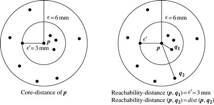
Figure 10.16 OPTICS terminology. Source: Based on Ankerst, Breunig, Kriegel, and Sander [ABKS99].
OPTICS computes an ordering of all objects in a given database and, for each object in the database, stores the core-distance and a suitable reachability-distance. OPTICS maintains a list called OrderSeeds to generate the output ordering. Objects in OrderSeeds are sorted by the reachability-distance from their respective closest core objects, that is, by the smallest reachability-distance of each object.
OPTICS begins with an arbitrary object from the input database as the current object, p. It retrieves the ![]() -neighborhood of p, determines the core-distance, and sets the reachability-distance to undefined. The current object, p, is then written to output. If p is not a core object, OPTICS simply moves on to the next object in the OrderSeeds list (or the input database if OrderSeeds is empty). If p is a core object, then for each object, q, in the
-neighborhood of p, determines the core-distance, and sets the reachability-distance to undefined. The current object, p, is then written to output. If p is not a core object, OPTICS simply moves on to the next object in the OrderSeeds list (or the input database if OrderSeeds is empty). If p is a core object, then for each object, q, in the ![]() -neighborhood of p, OPTICS updates its reachability-distance from p and inserts q into OrderSeeds if q has not yet been processed. The iteration continues until the input is fully consumed and OrderSeeds is empty.
-neighborhood of p, OPTICS updates its reachability-distance from p and inserts q into OrderSeeds if q has not yet been processed. The iteration continues until the input is fully consumed and OrderSeeds is empty.
A data set’s cluster ordering can be represented graphically, which helps to visualize and understand the clustering structure in a data set. For example, Figure 10.17 is the reachability plot for a simple 2-D data set, which presents a general overview of how the data are structured and clustered. The data objects are plotted in the clustering order (horizontal axis) together with their respective reachability-distances (vertical axis). The three Gaussian “bumps” in the plot reflect three clusters in the data set. Methods have also been developed for viewing clustering structures of high-dimensional data at various levels of detail.
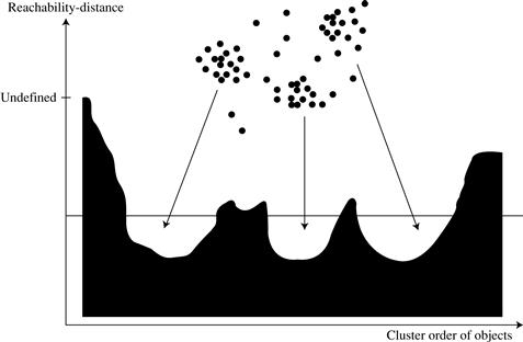
Figure 10.17 Cluster ordering in OPTICS. Source: Adapted from Ankerst, Breunig, Kriegel, and Sander [ABKS99].
The structure of the OPTICS algorithm is very similar to that of DBSCAN. Consequently, the two algorithms have the same time complexity. The complexity is O(n log n) if a spatial index is used, and O(n2) otherwise, where n is the number of objects.
10.4.3 DENCLUE: Clustering Based on Density Distribution Functions
Density estimation is a core issue in density-based clustering methods. DENCLUE (DENsity-based CLUstEring) is a clustering method based on a set of density distribution functions. We first give some background on density estimation, and then describe the DENCLUE algorithm.
In probability and statistics, density estimation is the estimation of an unobservable underlying probability density function based on a set of observed data. In the context of density-based clustering, the unobservable underlying probability density function is the true distribution of the population of all possible objects to be analyzed. The observed data set is regarded as a random sample from that population.
In DBSCAN and OPTICS, density is calculated by counting the number of objects in a neighborhood defined by a radius parameter, ![]() . Such density estimates can be highly sensitive to the radius value used. For example, in Figure 10.18, the density changes significantly as the radius increases by a small amount.
. Such density estimates can be highly sensitive to the radius value used. For example, in Figure 10.18, the density changes significantly as the radius increases by a small amount.
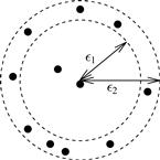
Figure 10.18 The subtlety in density estimation in DBSCAN and OPTICS: Increasing the neighborhood radius slightly from ![]() 1 to
1 to ![]() 2 results in a much higher density.
2 results in a much higher density.
To overcome this problem, kernel density estimation can be used, which is a nonparametric density estimation approach from statistics. The general idea behind kernel density estimation is simple. We treat an observed object as an indicator of high-probability density in the surrounding region. The probability density at a point depends on the distances from this point to the observed objects.
Formally, let x1, …, xn be an independent and identically distributed sample of a random variable f. The kernel density approximation of the probability density function is
![]() (10.21)
(10.21)
where K() is a kernel and h is the bandwidth serving as a smoothing parameter. A kernel can be regarded as a function modeling the influence of a sample point within its neighborhood. Technically, a kernel K() is a non-negative real-valued integrable function that should satisfy two requirements: ![]() and K(−u) = K(u) for all values of u. A frequently used kernel is a standard Gaussian function with a mean of 0 and a variance of 1:
and K(−u) = K(u) for all values of u. A frequently used kernel is a standard Gaussian function with a mean of 0 and a variance of 1:
![]() (10.22)
(10.22)
DENCLUE uses a Gaussian kernel to estimate density based on the given set of objects to be clustered. A point x* is called a density attractor if it is a local maximum of the estimated density function. To avoid trivial local maximum points, DENCLUE uses a noise threshold, ξ, and only considers those density attractors x* such that ![]() . These nontrivial density attractors are the centers of clusters.
. These nontrivial density attractors are the centers of clusters.
Objects under analysis are assigned to clusters through density attractors using a stepwise hill-climbing procedure. For an object, x, the hill-climbing procedure starts from x and is guided by the gradient of the estimated density function. That is, the density attractor for x is computed as
 (10.23)
where δ is a parameter to control the speed of convergence, and
![]() (10.24)
(10.24)
The hill-climbing procedure stops at step k > 0 if ![]() , and assigns x to the density attractor x* = xk. An object x is an outlier or noise if it converges in the hill-climbing procedure to a local maximum x* with
, and assigns x to the density attractor x* = xk. An object x is an outlier or noise if it converges in the hill-climbing procedure to a local maximum x* with ![]() .
.
A cluster in DENCLUE is a set of density attractors X and a set of input objects C such that each object in C is assigned to a density attractor in X, and there exists a path between every pair of density attractors where the density is above ξ. By using multiple density attractors connected by paths, DENCLUE can find clusters of arbitrary shape.
DENCLUE has several advantages. It can be regarded as a generalization of several well-known clustering methods such as single-linkage approaches and DBSCAN. Moreover, DENCLUE is invariant against noise. The kernel density estimation can effectively reduce the influence of noise by uniformly distributing noise into the input data.