
8.8 Exercises
8.1 Briefly outline the major steps of decision tree classification.
8.2 Why is tree pruning useful in decision tree induction? What is a drawback of using a separate set of tuples to evaluate pruning?
8.3 Given a decision tree, you have the option of (a) converting the decision tree to rules and then pruning the resulting rules, or (b) pruning the decision tree and then converting the pruned tree to rules. What advantage does (a) have over (b)?
8.4 It is important to calculate the worst-case computational complexity of the decision tree algorithm. Given data set, D, the number of attributes, n, and the number of training tuples, ![]() , show that the computational cost of growing a tree is at most
, show that the computational cost of growing a tree is at most ![]() .
.
8.5 Given a 5-GB data set with 50 attributes (each containing 100 distinct values) and 512 MB of main memory in your laptop, outline an efficient method that constructs decision trees in such large data sets. Justify your answer by rough calculation of your main memory usage.
8.6 Why is naïve Bayesian classification called “naïve”? Briefly outline the major ideas of naïve Bayesian classification.
8.7 The following table consists of training data from an employee database. The data have been generalized. For example, “31 … 35” for age represents the age range of 31 to 35. For a given row entry, count represents the number of data tuples having the values for department, status, age, and salary given in that row.
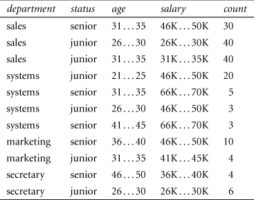
Let status be the class label attribute.
(a) How would you modify the basic decision tree algorithm to take into consideration the count of each generalized data tuple (i.e., of each row entry)?
(b) Use your algorithm to construct a decision tree from the given data.
(c) Given a data tuple having the values “systems," “26,” and “46–50K” for the attributes department, age, and salary, respectively, what would a naïve Bayesian classification of the status for the tuple be?
8.8 RainForest is a scalable algorithm for decision tree induction. Develop a scalable naïve Bayesian classification algorithm that requires just a single scan of the entire data set for most databases. Discuss whether such an algorithm can be refined to incorporate boosting to further enhance its classification accuracy.
8.9 Design an efficient method that performs effective naïve Bayesian classification over an infinite data stream (i.e., you can scan the data stream only once). If we wanted to discover the evolution of such classification schemes (e.g., comparing the classification scheme at this moment with earlier schemes such as one from a week ago), what modified design would you suggest?
8.10 Show that accuracy is a function of sensitivity and specificity, that is, prove Eq. (8.25).
8.11 The harmonic mean is one of several kinds of averages. Chapter 2 discussed how to compute the arithmetic mean, which is what most people typically think of when they compute an average. The harmonic mean, H, of the positive real numbers, ![]() , is defined as
, is defined as
The F measure is the harmonic mean of precision and recall. Use this fact to derive Eq. (8.28) for F. In addition, write ![]() as a function of true positives, false negatives, and false positives.
as a function of true positives, false negatives, and false positives.
8.12 The data tuples of Figure 8.25 are sorted by decreasing probability value, as returned by a classifier. For each tuple, compute the values for the number of true positives (TP), false positives (FP), true negatives (TN), and false negatives (FN). Compute the true positive rate (TPR) and false positive rate (FPR). Plot the ROC curve for the data.
8.13 It is difficult to assess classification accuracy when individual data objects may belong to more than one class at a time. In such cases, comment on what criteria you would use to compare different classifiers modeled after the same data.
8.14 Suppose that we want to select between two prediction models, M1 and M2. We have performed 10 rounds of 10-fold cross-validation on each model, where the same data partitioning in round i is used for both M1 and M2. The error rates obtained for M1 are 30.5, 32.2, 20.7, 20.6, 31.0, 41.0, 27.7, 26.0, 21.5, 26.0. The error rates for M2 are 22.4, 14.5, 22.4, 19.6, 20.7, 20.4, 22.1, 19.4, 16.2, 35.0. Comment on whether one model is significantly better than the other considering a significance level of 1%.
8.15 What is boosting? State why it may improve the accuracy of decision tree induction.
8.16 Outline methods for addressing the class imbalance problem. Suppose a bank wants to develop a classifier that guards against fraudulent credit card transactions. Illustrate how you can induce a quality classifier based on a large set of nonfraudulent examples and a very small set of fraudulent cases.
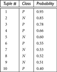
Figure 8.25 Tuples sorted by decreasing score, where the score is the value returned by a probabilistic classifier.