
7.5 Mining Compressed or Approximate Patterns
A major challenge in frequent pattern mining is the huge number of discovered patterns. Using a minimum support threshold to control the number of patterns found has limited effect. Too low a value can lead to the generation of an explosive number of output patterns, while too high a value can lead to the discovery of only commonsense patterns.
To reduce the huge set of frequent patterns generated in mining while maintaining high-quality patterns, we can instead mine a compressed or approximate set of frequent patterns. Top-k most frequent closed patterns were proposed to make the mining process concentrate on only the set of k most frequent patterns. Although interesting, they usually do not epitomize the k most representative patterns because of the uneven frequency distribution among itemsets. Constraint-based mining of frequent patterns (Section 7.3) incorporates user-specified constraints to filter out uninteresting patterns. Measures of pattern/rule interestingness and correlation (Section 6.3) can also be used to help confine the search to patterns/rules of interest.
In this section, we look at two forms of “compression” of frequent patterns that build on the concepts of closed patterns and max-patterns. Recall from Section 6.2.6 that a closed pattern is a lossless compression of the set of frequent patterns, whereas a max-pattern is a lossy compression. In particular, Section 7.5.1 explores clustering-based compression of frequent patterns, which groups patterns together based on their similarity and frequency support. Section 7.5.2 takes a “summarization” approach, where the aim is to derive redundancy-aware top-k representative patterns that cover the whole set of (closed) frequent itemsets. The approach considers not only the representativeness of patterns but also their mutual independence to avoid redundancy in the set of generated patterns. The k representatives provide compact compression over the collection of frequent patterns, making them easier to interpret and use.
7.5.1 Mining Compressed Patterns by Pattern Clustering
Pattern compression can be achieved by pattern clustering. Clustering techniques are described in detail in Chapters 10 and 11. In this section, it is not necessary to know the fine details of clustering. Rather, you will learn how the concept of clustering can be applied to compress frequent patterns. Clustering is the automatic process of grouping like objects together, so that objects within a cluster are similar to one another and dissimilar to objects in other clusters. In this case, the objects are frequent patterns. The frequent patterns are clustered using a tightness measure called δ-cluster. A representative pattern is selected for each cluster, thereby offering a compressed version of the set of frequent patterns.
Before we begin, let’s review some definitions. An itemset X is a closed frequent itemset in a data set D if X is frequent and there exists no proper super-itemset Y of X such that Y has the same support count as X in D. An itemset X is a maximal frequent itemset in data set D if X is frequent and there exists no super-itemset Y such that X ⊂ Y and Y is frequent in D. Using these concepts alone is not enough to obtain a good representative compression of a data set, as we see in Example 7.12.
So, let’s see if we can find a way of clustering frequent patterns as a means of obtaining a compressed representation of them. We will need to define a good similarity measure, cluster patterns according to this measure, and then select and output only a representative pattern for each cluster. Since the set of closed frequent patterns is a lossless compression over the original frequent patterns set, it is a good idea to discover representative patterns over the collection of closed patterns.
We can use the following distance measure between closed patterns. Let P1 and P2 be two closed patterns. Their supporting transaction sets are T(P1) and T(P2), respectively. The pattern distance of P1 and P2, Pat_Dist(P1, P2), is defined as
![]() (7.14)
(7.14)
Pattern distance is a valid distance metric defined on the set of transactions. Note that it incorporates the support information of patterns, as desired previously.
Example 7.13
Pattern distance
Suppose P1 and P2 are two patterns such that ![]() and
and ![]() , where ti is a transaction in the database. The distance between P1 and P2 is
, where ti is a transaction in the database. The distance between P1 and P2 is ![]() .
.
Now, let’s consider the expression of patterns. Given two patterns A and B, we say B can be expressed by A if O(B) ⊂ O(A), where O(A) is the corresponding itemset of pattern A. Following this definition, assume patterns ![]() are in the same cluster. The representative pattern Pr of the cluster should be able to express all the other patterns in the cluster. Clearly, we have
are in the same cluster. The representative pattern Pr of the cluster should be able to express all the other patterns in the cluster. Clearly, we have ![]() .
.
Using the distance measure, we can simply apply a clustering method, such as k-means (Section 10.2), on the collection of frequent patterns. However, this introduces two problems. First, the quality of the clusters cannot be guaranteed; second, it may not be able to find a representative pattern for each cluster (i.e., the pattern Pr may not belong to the same cluster). To overcome these problems, this is where the concept of δ-cluster comes in, where δ (0 ≤ δ ≤ 1) measures the tightness of a cluster.
A pattern P is δ-covered by another pattern P′ if ![]() and Pat_Dist(P, P′) ≤ δ. A set of patterns form a δ-cluster if there exists a representative pattern Pr such that for each pattern P in the set, P is δ-covered by Pr.
and Pat_Dist(P, P′) ≤ δ. A set of patterns form a δ-cluster if there exists a representative pattern Pr such that for each pattern P in the set, P is δ-covered by Pr.
Note that according to the concept of δ-cluster, a pattern can belong to multiple clusters. Also, using δ-cluster, we only need to compute the distance between each pattern and the representative pattern of the cluster. Because a pattern P is δ-covered by a representative pattern Pr only if ![]() , we can simplify the distance calculation by considering only the supports of the patterns:
, we can simplify the distance calculation by considering only the supports of the patterns:
![]() (7.15)
(7.15)
If we restrict the representative pattern to be frequent, then the number of representative patterns (i.e., clusters) is no less than the number of maximal frequent patterns. This is because a maximal frequent pattern can only be covered by itself. To achieve more succinct compression, we relax the constraints on representative patterns, that is, we allow the support of representative patterns to be somewhat less than min_sup.
For any representative pattern Pr, assume its support is k. Since it has to cover at least one frequent pattern (i.e., P) with support that is at least min_sup, we have
![]() (7.16)
(7.16)
That is, k ≥ (1 − δ) × min_sup. This is the minimum support for a representative pattern, denoted as min_supr.
Based on the preceding discussion, the pattern compression problem can be defined as follows: Given a transaction database, a minimum support min_sup, and the cluster quality measure δ, the pattern compression problem is to find a set of representative patterns R such that for each frequent pattern P (with respect to min_sup), there is a representative pattern Pr ∈ R (with respect to min_supr), which covers P, and the value of |R| is minimized.
Finding a minimum set of representative patterns is an NP-Hard problem. However, efficient methods have been developed that reduce the number of closed frequent patterns generated by orders of magnitude with respect to the original collection of closed patterns. The methods succeed in finding a high-quality compression of the pattern set.
7.5.2 Extracting Redundancy-Aware Top-k Patterns
Mining the top-k most frequent patterns is a strategy for reducing the number of patterns returned during mining. However, in many cases, frequent patterns are not mutually independent but often clustered in small regions. This is somewhat like finding 20 population centers in the world, which may result in cities clustered in a small number of countries rather than evenly distributed across the globe. Instead, most users would prefer to derive the k most interesting patterns, which are not only significant, but also mutually independent and containing little redundancy. A small set of k representative patterns that have not only high significance but also low redundancy are called redundancy-aware top-k patterns.
Example 7.14
Redundancy-aware top-k strategy versus other top-k strategies
Figure 7.11 illustrates the intuition behind redundancy-aware top-k patterns versus traditional top-k patterns and k-summarized patterns. Suppose we have the frequent patterns set shown in Figure 7.11(a), where each circle represents a pattern of which the significance is colored in grayscale. The distance between two circles reflects the redundancy of the two corresponding patterns: The closer the circles are, the more redundant the respective patterns are to one another. Let’s say we want to find three patterns that will best represent the given set, that is, k = 3. Which three should we choose?
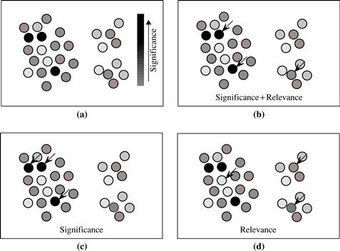
Figure 7.11 Conceptual view comparing top-k methodologies (where gray levels represent pattern significance, and the closer that two patterns are displayed, the more redundant they are to one another): (a) original patterns, (b) redundancy-aware top-k patterns, (c) traditional top-k patterns, and (d) k-summarized patterns.
Arrows are used to show the patterns chosen if using redundancy-aware top-k patterns (Figure 7.11b), traditional top-k patterns (Figure 7.11c), or k-summarized patterns (Figure 7.11d). In Figure 7.11(c), the traditional top-k strategy relies solely on significance: It selects the three most significant patterns to represent the set.
In Figure 7.11(d), the k-summarized pattern strategy selects patterns based solely on nonredundancy. It detects three clusters, and finds the most representative patterns to be the “centermost’” pattern from each cluster. These patterns are chosen to represent the data. The selected patterns are considered “summarized patterns” in the sense that they represent or “provide a summary” of the clusters they stand for.
By contrast, in Figure 7.11(b) the redundancy-aware top-k patterns make a trade-off between significance and redundancy. The three patterns chosen here have high significance and low redundancy. Observe, for example, the two highly significant patterns that, based on their redundancy, are displayed next to each other. The redundancy-aware top-k strategy selects only one of them, taking into consideration that two would be redundant. To formalize the definition of redundancy-aware top-k patterns, we’ll need to define the concepts of significance and redundancy.
A significance measure S is a function mapping a pattern ![]() to a real value such that S(p) is the degree of interestingness (or usefulness) of the pattern p. In general, significance measures can be either objective or subjective. Objective measures depend only on the structure of the given pattern and the underlying data used in the discovery process. Commonly used objective measures include support, confidence, correlation, and tf-idf (or term frequency versus inverse document frequency), where the latter is often used in information retrieval. Subjective measures are based on user beliefs in the data. They therefore depend on the users who examine the patterns. A subjective measure is usually a relative score based on user prior knowledge or a background model. It often measures the unexpectedness of a pattern by computing its divergence from the background model. Let S(p, q) be the combined significance of patterns p and q, and
to a real value such that S(p) is the degree of interestingness (or usefulness) of the pattern p. In general, significance measures can be either objective or subjective. Objective measures depend only on the structure of the given pattern and the underlying data used in the discovery process. Commonly used objective measures include support, confidence, correlation, and tf-idf (or term frequency versus inverse document frequency), where the latter is often used in information retrieval. Subjective measures are based on user beliefs in the data. They therefore depend on the users who examine the patterns. A subjective measure is usually a relative score based on user prior knowledge or a background model. It often measures the unexpectedness of a pattern by computing its divergence from the background model. Let S(p, q) be the combined significance of patterns p and q, and ![]() be the relative significance of p given q. Note that the combined significance, S(p, q), means the collective significance of two individual patterns p and q, not the significance of a single super pattern p ∪ q.
be the relative significance of p given q. Note that the combined significance, S(p, q), means the collective significance of two individual patterns p and q, not the significance of a single super pattern p ∪ q.
Given the significance measure S, the redundancy R between two patterns p and q is defined as ![]() . Subsequently, we have
. Subsequently, we have ![]() .
.
We assume that the combined significance of two patterns is no less than the significance of any individual pattern (since it is a collective significance of two patterns) and does not exceed the sum of two individual significance patterns (since there exists redundancy). That is, the redundancy between two patterns should satisfy
![]() (7.17)
(7.17)
The ideal redundancy measure R(p, q) is usually hard to obtain. However, we can approximate redundancy using distance between patterns such as with the distance measure defined in Section 7.5.1.
The problem of finding redundancy-aware top-k patterns can thus be transformed into finding a k-pattern set that maximizes the marginal significance, which is a well-studied problem in information retrieval. In this field, a document has high marginal relevance if it is both relevant to the query and contains minimal marginal similarity to previously selected documents, where the marginal similarity is computed by choosing the most relevant selected document. Experimental studies have shown this method to be efficient and able to find high-significance and low-redundancy top-k patterns.