
5.4 Multidimensional Data Analysis in Cube Space
Data cubes create a flexible and powerful means to group and aggregate data subsets. They allow data to be explored in multiple dimensional combinations and at varying aggregate granularities. This capability greatly increases the analysis bandwidth and helps effective discovery of interesting patterns and knowledge from data. The use of cube space makes the data space both meaningful and tractable.
This section presents methods of multidimensional data analysis that make use of data cubes to organize data into intuitive regions of interest at varying granularities. Section 5.4.1 presents prediction cubes, a technique for multidimensional data mining that facilitates predictive modeling in multidimensional space. Section 5.4.2 describes how to construct multifeature cubes. These support complex analytical queries involving multiple dependent aggregates at multiple granularities. Finally, Section 5.4.3 describes an interactive method for users to systematically explore cube space. In such exception-based, discovery-driven exploration, interesting exceptions or anomalies in the data are automatically detected and marked for users with visual cues.
5.4.1 Prediction Cubes: Prediction Mining in Cube Space
Recently, researchers have turned their attention toward multidimensional data mining to uncover knowledge at varying dimensional combinations and granularities. Such mining is also known as exploratory multidimensional data mining and online analytical data mining (OLAM). Multidimensional data space is huge. In preparing the data, how can we identify the interesting subspaces for exploration? To what granularities should we aggregate the data? Multidimensional data mining in cube space organizes data of interest into intuitive regions at various granularities. It analyzes and mines the data by applying various data mining techniques systematically over these regions.
There are at least four ways in which OLAP-style analysis can be fused with data mining techniques:
1. Use cube space to define the data space for mining. Each region in cube space represents a subset of data over which we wish to find interesting patterns. Cube space is defined by a set of expert-designed, informative dimension hierarchies, not just arbitrary subsets of data. Therefore, the use of cube space makes the data space both meaningful and tractable.
2. Use OLAP queries to generate features and targets for mining. The features and even the targets (that we wish to learn to predict) can sometimes be naturally defined as OLAP aggregate queries over regions in cube space.
3. Use data mining models as building blocks in a multistep mining process. may consist of multiple steps, where data mining models can be viewed as building blocks that are used to describe the behavior of interesting data sets, rather than the end results.
4. Use data cube computation techniques to speed up repeated model construction. may require building a model for each candidate data space, which is usually too expensive to be feasible. However, by carefully sharing computation across model construction for different candidates based on data cube computation techniques, efficient mining is achievable.
In this subsection we study prediction cubes, an example of multidimensional data mining where the cube space is explored for prediction tasks. A prediction cube is a cube structure that stores prediction models in multidimensional data space and supports prediction in an OLAP manner. Recall that in a data cube, each cell value is an aggregate number (e.g., count) computed over the data subset in that cell. However, each cell value in a prediction cube is computed by evaluating a predictive model built on the data subset in that cell, thereby representing that subset’s predictive behavior.
Instead of seeing prediction models as the end result, prediction cubes use prediction models as building blocks to define the interestingness of data subsets, that is, they identify data subsets that indicate more accurate prediction. This is best explained with an example.
Example 5.18
Prediction cube for identification of interesting cube subspaces
Suppose a company has a customer table with the attributes time (with two granularity levels: month and year), location (with two granularity levels: state and country), gender, salary, and one class-label attribute: valued_customer. A manager wants to analyze the decision process of whether a customer is highly valued with respect to time and location. In particular, he is interested in the question “Are there times at and locations in which the value of a customer depended greatly on the customer’s gender?” Notice that he believes time and location play a role in predicting valued customers, but at what granularity levels do they depend on gender for this task? For example, is performing analysis using {month, country} better than {year, state}?
Consider a data table D (e.g., the customer table). Let X be the (e.g., gender, salary). Let Y be the class-label attribute (e.g., valued_customer), and Z be the set of attributes, that is, attributes for which concept hierarchies have been defined (e.g., time, location). Let V be the set of attributes for which we would like to define their predictiveness. In our example, this set is {gender}. The predictiveness of V on a data subset can be quantified by the difference in accuracy between the model built on that subset using X to predict Y and the model built on that subset using X − V (e.g., {salary}) to predict Y. The intuition is that, if the difference is large, V must play an important role in the prediction of class label Y.
Given a set of attributes, V, and a learning algorithm, the cube at granularity ![]() (e.g.,
(e.g., ![]() ) is a d-dimensional array, in which the value in each cell (e.g., [2010, Illinois]) is the predictiveness of V evaluated on the subset defined by the cell (e.g., the records in the customer table with time in 2010 and location in Illinois).
) is a d-dimensional array, in which the value in each cell (e.g., [2010, Illinois]) is the predictiveness of V evaluated on the subset defined by the cell (e.g., the records in the customer table with time in 2010 and location in Illinois).
Supporting OLAP roll-up and drill-down operations on a prediction cube is a computational challenge requiring the materialization of cell values at many different granularities. For simplicity, we can consider only full materialization. A na ve way to fully materialize a prediction cube is to exhaustively build models and evaluate them for each cell and granularity. This method is very expensive if the base data set is large. An ensemble method called Probability-Based Ensemble (PBE) was developed as a more feasible alternative. It requires model construction for only the finest-grained cells. OLAP-style bottom-up aggregation is then used to generate the values of the coarser-grained cells.
The prediction of a predictive model can be seen as finding a class label that maximizes a scoring function. The PBE method was developed to approximately make the scoring function of any predictive model distributively decomposable. In our discussion of data cube measures in Section 4.2.4, we showed that distributive and algebraic measures can be computed efficiently. Therefore, if the scoring function used is distributively or algebraically decomposable, prediction cubes can also be computed with efficiency. In this way, the PBE method reduces prediction cube computation to data cube computation.
For example, previous studies have shown that the naïve Bayes classifier has an algebraically decomposable scoring function, and the kernel density–based classifier has a distributively decomposable scoring function.8 Therefore, either of these could be used to implement prediction cubes efficiently. The PBE method presents a novel approach to multidimensional data mining in cube space.
5.4.2 Multifeature Cubes: Complex Aggregation at Multiple Granularities
Data cubes facilitate the answering of queries as they allow the computation of aggregate data at multiple granularity levels. Traditional data cubes are typically constructed on commonly used dimensions (e.g., time, location, and product) using simple measures (e.g., count(), average(), and sum()). In this section, you will learn a newer way to define data cubes called multifeature cubes. Multifeature cubes enable more in-depth analysis. They can compute more complex queries of which the measures depend on groupings of multiple aggregates at varying granularity levels. The queries posed can be much more elaborate and task-specific than traditional queries, as we shall illustrate in the next examples. Many complex data mining queries can be answered by multifeature cubes without significant increase in computational cost, in comparison to cube computation for simple queries with traditional data cubes.
To illustrate the idea of multifeature cubes, let’s first look at an example of a query on a simple data cube.
To illustrate what is meant by “dependent aggregates,” let’s examine a more complex query, which can be computed with a multifeature cube.
“How can multifeature cubes be computed efficiently?” The computation of a multifeature cube depends on the types of aggregate functions used in the cube. In Chapter 4, we saw that aggregate functions can be categorized as either distributive, algebraic, or holistic. Multifeature cubes can be organized into the same categories and computed efficiently by minor extension of the cube computation methods in Section 5.2.
5.4.3 Exception-Based, Discovery-Driven Cube Space Exploration
As studied in previous sections, a data cube may have a large number of cuboids, and each cuboid may contain a large number of (aggregate) cells. With such an overwhelmingly large space, it becomes a burden for users to even just browse a cube, let alone think of exploring it thoroughly. Tools need to be developed to assist users in intelligently exploring the huge aggregated space of a data cube.
In this section, we describe a discovery-driven approach to exploring cube space. Precomputed measures indicating data exceptions are used to guide the user in the data analysis process, at all aggregation levels. We hereafter refer to these measures as exception indicators. Intuitively, an exception is a data cube cell value that is significantly different from the value anticipated, based on a statistical model. The model considers variations and patterns in the measure value across all the dimensions to which a cell belongs. For example, if the analysis of item-sales data reveals an increase in sales in December in comparison to all other months, this may seem like an exception in the time dimension. However, it is not an exception if the item dimension is considered, since there is a similar increase in sales for other items during December.
The model considers exceptions hidden at all aggregated group-by’s of a data cube. Visual cues, such as background color, are used to reflect each cell’s degree of exception, based on the precomputed exception indicators. Efficient algorithms have been proposed for cube construction, as discussed in Section 5.2. The computation of exception indicators can be overlapped with cube construction, so that the overall construction of data cubes for discovery-driven exploration is efficient.
Three measures are used as exception indicators to help identify data anomalies. These measures indicate the degree of surprise that the quantity in a cell holds, with respect to its expected value. The measures are computed and associated with every cell, for all aggregation levels. They are as follows:
■ SelfExp: This indicates the degree of surprise of the cell value, relative to other cells at the same aggregation level.
■ InExp: This indicates the degree of surprise somewhere beneath the cell, if we were to drill down from it.
■ PathExp: This indicates the degree of surprise for each drill-down path from the cell.
The use of these measures for discovery-driven exploration of data cubes is illustrated in Example 5.21.
Example 5.21
Discovery-driven exploration of a data cube
Suppose that you want to analyze the monthly sales at AllElectronics as a percentage difference from the previous month. The dimensions involved are item, time, and region. You begin by studying the data aggregated over all items and sales regions for each month, as shown in Figure 5.16.
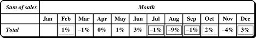
To view the exception indicators, you click on a button marked highlight exceptions on the screen. This translates the SelfExp and InExp values into visual cues, displayed with each cell. Each cell’s background color is based on its SelfExp value. In addition, a box is drawn around each cell, where the thickness and color of the box are functions of its InExp value. Thick boxes indicate high InExp values. In both cases, the darker the color, the greater the degree of exception. For example, the dark, thick boxes for sales during July, August, and September signal the user to explore the lower-level aggregations of these cells by drilling down.
Drill-downs can be executed along the aggregated item or region dimensions. “Which path has more exceptions?” you wonder. To find this out, you select a cell of interest and trigger a path exception module that colors each dimension based on the PathExp value of the cell. This value reflects that path’s degree of surprise. Suppose that the path along item contains more exceptions.
A drill-down along item results in the cube slice of Figure 5.17, showing the sales over time for each item. At this point, you are presented with many different sales values to analyze. By clicking on the highlight exceptions button, the visual cues are displayed, bringing focus to the exceptions. Consider the sales difference of 41% for “Sony b/w printers” in September. This cell has a dark background, indicating a high SelfExp value, meaning that the cell is an exception. Consider now the sales difference of −15% for “Sony b/w printers” in November and of −11% in December. The −11% value for December is marked as an exception, while the −15% value is not, even though −15% is a bigger deviation than −11%. This is because the exception indicators consider all the dimensions that a cell is in. Notice that the December sales of most of the other items have a large positive value, while the November sales do not. Therefore, by considering the cell’s position in the cube, the sales difference for “Sony b/w printers” in December is exceptional, while the November sales difference of this item is not.
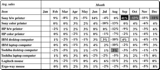
The InExp values can be used to indicate exceptions at lower levels that are not visible at the current level. Consider the cells for “IBM desktop computers” in July and September. These both have a dark, thick box around them, indicating high InExp values. You may decide to further explore the sales of “IBM desktop computers” by drilling down along region. The resulting sales difference by region is shown in Figure 5.18, where the highlight exceptions option has been invoked. The visual cues displayed make it easy to instantly notice an exception for the sales of “IBM desktop computers” in the southern region, where such sales have decreased by −39% and −34% in July and September, respectively. These detailed exceptions were far from obvious when we were viewing the data as an item-time group-by, aggregated over region in Figure 5.17. Thus, the InExp value is useful for searching for exceptions at lower-level cells of the cube.

“How are the exception values computed?” The SelfExp, InExp, and PathExp measures are based on a statistical method for table analysis. They take into account all of the group-by’s (aggregations) in which a given cell value participates. A cell value is considered an exception based on how much it differs from its expected value, where its expected value is determined with a statistical model. The difference between a given cell value and its expected value is called a residual. Intuitively, the larger the residual, the more the given cell value is an exception. The comparison of residual values requires us to scale the values based on the expected standard deviation associated with the residuals. A cell value is therefore considered an exception if its scaled residual value exceeds a prespecified threshold. The SelfExp, InExp, and PathExp measures are based on this scaled residual.
The expected value of a given cell is a function of the higher-level group-by’s of the given cell. For example, given a cube with the three dimensions A, B, and C, the expected value for a cell at the i th position in A, the j th position in B, and the kth position in C is a function of ![]() , and
, and ![]() , which are coefficients of the statistical model used. The coefficients reflect how different the values at more detailed levels are, based on generalized impressions formed by looking at higher-level aggregations. In this way, the exception quality of a cell value is based on the exceptions of the values below it. Thus, when seeing an exception, it is natural for the user to further explore the exception by drilling down.
, which are coefficients of the statistical model used. The coefficients reflect how different the values at more detailed levels are, based on generalized impressions formed by looking at higher-level aggregations. In this way, the exception quality of a cell value is based on the exceptions of the values below it. Thus, when seeing an exception, it is natural for the user to further explore the exception by drilling down.
“How can the data cube be efficiently constructed for discovery-driven exploration?” This computation consists of three phases. The first step involves the computation of the aggregate values defining the cube, such as sum or count, over which exceptions will be found. The second phase consists of model fitting, in which the coefficients mentioned before are determined and used to compute the standardized residuals. This phase can be overlapped with the first phase because the computations involved are similar. The third phase computes the SelfExp, InExp, and PathExp values, based on the standardized residuals. This phase is computationally similar to phase 1. Therefore, the computation of data cubes for discovery-driven exploration can be done efficiently.