
3.3 Data Integration
Data mining often requires data integration—the merging of data from multiple data stores. Careful integration can help reduce and avoid redundancies and inconsistencies in the resulting data set. This can help improve the accuracy and speed of the subsequent data mining process.
The semantic heterogeneity and structure of data pose great challenges in data integration. How can we match schema and objects from different sources? This is the essence of the entity identification problem, described in Section 3.3.1. Are any attributes correlated? Section 3.3.2 presents correlation tests for numeric and nominal data. Tuple duplication is described in Section 3.3.3. Finally, Section 3.3.4 touches on the detection and resolution of data value conflicts.
3.3.1 Entity Identification Problem
It is likely that your data analysis task will involve data integration, which combines data from multiple sources into a coherent data store, as in data warehousing. These sources may include multiple databases, data cubes, or flat files.
There are a number of issues to consider during data integration. Schema integration and object matching can be tricky. How can equivalent real-world entities from multiple data sources be matched up? This is referred to as the entity identification problem. For example, how can the data analyst or the computer be sure that customer_id in one database and cust_number in another refer to the same attribute? Examples of metadata for each attribute include the name, meaning, data type, and range of values permitted for the attribute, and null rules for handling blank, zero, or null values (Section 3.2). Such metadata can be used to help avoid errors in schema integration. The metadata may also be used to help transform the data (e.g., where data codes for pay_type in one database may be “H” and “S” but 1 and 2 in another). Hence, this step also relates to data cleaning, as described earlier.
When matching attributes from one database to another during integration, special attention must be paid to the structure of the data. This is to ensure that any attribute functional dependencies and referential constraints in the source system match those in the target system. For example, in one system, a discount may be applied to the order, whereas in another system it is applied to each individual line item within the order. If this is not caught before integration, items in the target system may be improperly discounted.
3.3.2 Redundancy and Correlation Analysis
Redundancy is another important issue in data integration. An attribute (such as annual revenue, for instance) may be redundant if it can be “derived” from another attribute or set of attributes. Inconsistencies in attribute or dimension naming can also cause redundancies in the resulting data set.
Some redundancies can be detected by correlation analysis. Given two attributes, such analysis can measure how strongly one attribute implies the other, based on the available data. For nominal data, we use the χ2 (chi-square) test. For numeric attributes, we can use the correlation coefficient and covariance, both of which access how one attribute’s values vary from those of another.
χ2 Correlation Test for Nominal Data
For nominal data, a correlation relationship between two attributes, A and B, can be discovered by a χ2 (chi-square) test. Suppose A has c distinct values, namely a1, a2, … ac. B has r distinct values, namely b1, b2, … br. The data tuples described by A and B can be shown as a contingency table, with the c values of A making up the columns and the r values of B making up the rows. Let (Ai, Bj) denote the joint event that attribute A takes on value ai and attribute B takes on value bj, that is, where (A = ai, B = bj). Each and every possible (Ai, Bj) joint event has its own cell (or slot) in the table. The χ2 value (also known as the Pearson χ2 statistic) is computed as
![]() (3.1)
(3.1)
where oij is the observed frequency (i.e., actual count) of the joint event (Ai, Bj) and eij is the expected frequency of (Ai, Bj), which can be computed as
![]() (3.2)
(3.2)
where n is the number of data tuples, count(A = ai) is the number of tuples having value ai for A, and count(B = bj) is the number of tuples having value bj for B. The sum in Eq. (3.1) is computed over all of the r × c cells. Note that the cells that contribute the most to the χ2 value are those for which the actual count is very different from that expected.
The χ2 statistic tests the hypothesis that A and B are independent, that is, there is no correlation between them. The test is based on a significance level, with (r − 1) × (c − 1) degrees of freedom. We illustrate the use of this statistic in Example 3.1. If the hypothesis can be rejected, then we say that A and B are statistically correlated.
Example 3.1
Correlation analysis of nominal attributes using χ2
Suppose that a group of 1500 people was surveyed. The gender of each person was noted. Each person was polled as to whether his or her preferred type of reading material was fiction or nonfiction. Thus, we have two attributes, gender and preferred_reading. The observed frequency (or count) of each possible joint event is summarized in the contingency table shown in Table 3.1, where the numbers in parentheses are the expected frequencies. The expected frequencies are calculated based on the data distribution for both attributes using Eq. (3.2).
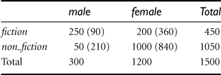
Using Eq. (3.2), we can verify the expected frequencies for each cell. For example, the expected frequency for the cell (male, fiction) is
![]()
and so on. Notice that in any row, the sum of the expected frequencies must equal the total observed frequency for that row, and the sum of the expected frequencies in any column must also equal the total observed frequency for that column.
Using Eq. (3.1) for χ2 computation, we get
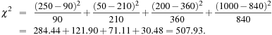
For this 2 × 2 table, the degrees of freedom are (2 − 1)(2 − 1) = 1. For 1 degree of freedom, the χ2 value needed to reject the hypothesis at the 0.001 significance level is 10.828 (taken from the table of upper percentage points of the χ2 distribution, typically available from any textbook on statistics). Since our computed value is above this, we can reject the hypothesis that gender and preferred_reading are independent and conclude that the two attributes are (strongly) correlated for the given group of people.
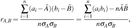
Correlation Coefficient for Numeric Data
For numeric attributes, we can evaluate the correlation between two attributes, A and B, by computing the correlation coefficient (also known as Pearson’s product moment coefficient, named after its inventer, Karl Pearson). This is
 (3.3)
(3.3)
where n is the number of tuples, ai and bi are the respective values of A and B in tuple i, Ā and ![]() are the respective mean values of A and B, σA and σB are the respective standard deviations of A and B (as defined in Section 2.2.2), and Σ(aibi) is the sum of the AB cross-product (i.e., for each tuple, the value for A is multiplied by the value for B in that tuple). Note that −1 ≤ rA, B ≤ +1. If rA, B is greater than 0, then A and B are positively correlated, meaning that the values of A increase as the values of B increase. The higher the value, the stronger the correlation (i.e., the more each attribute implies the other). Hence, a higher value may indicate that A (or B) may be removed as a redundancy.
are the respective mean values of A and B, σA and σB are the respective standard deviations of A and B (as defined in Section 2.2.2), and Σ(aibi) is the sum of the AB cross-product (i.e., for each tuple, the value for A is multiplied by the value for B in that tuple). Note that −1 ≤ rA, B ≤ +1. If rA, B is greater than 0, then A and B are positively correlated, meaning that the values of A increase as the values of B increase. The higher the value, the stronger the correlation (i.e., the more each attribute implies the other). Hence, a higher value may indicate that A (or B) may be removed as a redundancy.
If the resulting value is equal to 0, then A and B are independent and there is no correlation between them. If the resulting value is less than 0, then A and B are negatively correlated, where the values of one attribute increase as the values of the other attribute decrease. This means that each attribute discourages the other. Scatter plots can also be used to view correlations between attributes (Section 2.2.3). For example, Figure 2.8’s scatter plots respectively show positively correlated data and negatively correlated data, while Figure 2.9 displays uncorrelated data.
Note that correlation does not imply causality. That is, if A and B are correlated, this does not necessarily imply that A causes B or that B causes A. For example, in analyzing a demographic database, we may find that attributes representing the number of hospitals and the number of car thefts in a region are correlated. This does not mean that one causes the other. Both are actually causally linked to a third attribute, namely, population.
Covariance of Numeric Data
In probability theory and statistics, correlation and covariance are two similar measures for assessing how much two attributes change together. Consider two numeric attributes A and B, and a set of n observations {(a1, b1), …, (an, bn)}. The mean values of A and B, respectively, are also known as the expected values on A and B, that is,
![]()
and
![]()
The covariance between A and B is defined as
![]() (3.4)
(3.4)
If we compare Eq. (3.3) for rA, B (correlation coefficient) with Eq. (3.4) for covariance, we see that
![]() (3.5)
(3.5)
where σA and σB are the standard deviations of A and B, respectively. It can also be shown that
![]() (3.6)
(3.6)
This equation may simplify calculations.
For two attributes A and B that tend to change together, if A is larger than Ā (the expected value of A), then B is likely to be larger than ![]() (the expected value of B). Therefore, the covariance between A and B is positive. On the other hand, if one of the attributes tends to be above its expected value when the other attribute is below its expected value, then the covariance of A and B is negative.
(the expected value of B). Therefore, the covariance between A and B is positive. On the other hand, if one of the attributes tends to be above its expected value when the other attribute is below its expected value, then the covariance of A and B is negative.
If A and B are independent (i.e., they do not have correlation), then E(A ⋅ B) = E(A) ⋅ E(B). Therefore, the covariance is ![]() . However, the converse is not true. Some pairs of random variables (attributes) may have a covariance of 0 but are not independent. Only under some additional assumptions (e.g., the data follow multivariate normal distributions) does a covariance of 0 imply independence.
. However, the converse is not true. Some pairs of random variables (attributes) may have a covariance of 0 but are not independent. Only under some additional assumptions (e.g., the data follow multivariate normal distributions) does a covariance of 0 imply independence.
Example 3.2
Covariance analysis of numeric attributes
Consider Table 3.2, which presents a simplified example of stock prices observed at five time points for AllElectronics and HighTech, a high-tech company. If the stocks are affected by the same industry trends, will their prices rise or fall together?
![]()
and
![]()
Thus, using Eq. (3.4), we compute
![]()
Therefore, given the positive covariance we can say that stock prices for both companies rise together.
Variance is a special case of covariance, where the two attributes are identical (i.e., the covariance of an attribute with itself). Variance was discussed in Chapter 2.
3.3.3 Tuple Duplication
In addition to detecting redundancies between attributes, duplication should also be detected at the tuple level (e.g., where there are two or more identical tuples for a given unique data entry case). The use of denormalized tables (often done to improve performance by avoiding join s) is another source of data redundancy. Inconsistencies often arise between various duplicates, due to inaccurate data entry or updating some but not all data occurrences. For example, if a purchase order database contains attributes for the purchaser’s name and address instead of a key to this information in a purchaser database, discrepancies can occur, such as the same purchaser’s name appearing with different addresses within the purchase order database.
3.3.4 Data Value Conflict Detection and Resolution
Data integration also involves the detection and resolution of data value conflicts. For example, for the same real-world entity, attribute values from different sources may differ. This may be due to differences in representation, scaling, or encoding. For instance, a weight attribute may be stored in metric units in one system and British imperial units in another. For a hotel chain, the price of rooms in different cities may involve not only different currencies but also different services (e.g., free breakfast) and taxes. When exchanging information between schools, for example, each school may have its own curriculum and grading scheme. One university may adopt a quarter system, offer three courses on database systems, and assign grades from A+ to F, whereas another may adopt a semester system, offer two courses on databases, and assign grades from 1 to 10. It is difficult to work out precise course-to-grade transformation rules between the two universities, making information exchange difficult.
Attributes may also differ on the abstraction level, where an attribute in one system is recorded at, say, a lower abstraction level than the “same” attribute in another. For example, the total_sales in one database may refer to one branch of All_Electronics, while an attribute of the same name in another database may refer to the total sales for All_Electronics stores in a given region. The topic of discrepancy detection is further described in Section 3.2.3 on data cleaning as a process.