
9.4 Classification Using Frequent Patterns
Frequent patterns show interesting relationships between attribute–value pairs that occur frequently in a given data set. For example, we may find that the attribute–value pairs ![]() and
and ![]() occur in 20% of data tuples describing AllElectronics customers who buy a computer. We can think of each attribute–value pair as an item, so the search for these frequent patterns is known as frequent pattern mining or frequent itemset mining. In Chapters 6 and 7, we saw how association rules are derived from frequent patterns, where the associations are commonly used to analyze the purchasing patterns of customers in a store. Such analysis is useful in many decision-making processes such as product placement, catalog design, and cross-marketing.
occur in 20% of data tuples describing AllElectronics customers who buy a computer. We can think of each attribute–value pair as an item, so the search for these frequent patterns is known as frequent pattern mining or frequent itemset mining. In Chapters 6 and 7, we saw how association rules are derived from frequent patterns, where the associations are commonly used to analyze the purchasing patterns of customers in a store. Such analysis is useful in many decision-making processes such as product placement, catalog design, and cross-marketing.
In this section, we examine how frequent patterns can be used for classification. Section 9.4.1 explores associative classification, where association rules are generated from frequent patterns and used for classification. The general idea is that we can search for strong associations between frequent patterns (conjunctions of attribute–value pairs) and class labels. Section 9.4.2 explores discriminative frequent pattern–based classification, where frequent patterns serve as combined features, which are considered in addition to single features when building a classification model. Because frequent patterns explore highly confident associations among multiple attributes, frequent pattern–based classification may overcome some constraints introduced by decision tree induction, which considers only one attribute at a time. Studies have shown many frequent pattern–based classification methods to have greater accuracy and scalability than some traditional classification methods such as C4.5.
9.4.1 Associative Classification
In this section, you will learn about associative classification. The methods discussed are CBA, CMAR, and CPAR.
Before we begin, however, let’s look at association rule mining in general. Association rules are mined in a two-step process consisting of frequent itemset mining followed by rule generation. The first step searches for patterns of attribute–value pairs that occur repeatedly in a data set, where each attribute–value pair is considered an item. The resulting attribute–value pairs form frequent itemsets (also referred to as frequent patterns). The second step analyzes the frequent itemsets to generate association rules. All association rules must satisfy certain criteria regarding their “accuracy” (or confidence) and the proportion of the data set that they actually represent (referred to as support). For example, the following is an association rule mined from a data set, D, shown with its confidence and support:
![]() (9.21)
(9.21)
where ∧ represents a logical “AND.” We will say more about confidence and support later.
More formally, let D be a data set of tuples. Each tuple in D is described by n attributes, ![]() , and a class label attribute,
, and a class label attribute, ![]() . All continuous attributes are discretized and treated as categorical (or nominal) attributes. An item, p, is an attribute–value pair of the form (
. All continuous attributes are discretized and treated as categorical (or nominal) attributes. An item, p, is an attribute–value pair of the form (![]() ), where Ai is an attribute taking a value, v. A data tuple
), where Ai is an attribute taking a value, v. A data tuple ![]() satisfies an item,
satisfies an item, ![]() , if and only if
, if and only if ![]() , where xi is the value of the i th attribute of X. Association rules can have any number of items in the rule antecedent (left side) and any number of items in the rule consequent (right side). However, when mining association rules for use in classification, we are only interested in association rules of the form
, where xi is the value of the i th attribute of X. Association rules can have any number of items in the rule antecedent (left side) and any number of items in the rule consequent (right side). However, when mining association rules for use in classification, we are only interested in association rules of the form ![]() , where the rule antecedent is a conjunction of items,
, where the rule antecedent is a conjunction of items, ![]() (
(![]() ), associated with a class label, C. For a given rule, R, the percentage of tuples in D satisfying the rule antecedent that also have the class label C is called the confidence of R.
), associated with a class label, C. For a given rule, R, the percentage of tuples in D satisfying the rule antecedent that also have the class label C is called the confidence of R.
From a classification point of view, this is akin to rule accuracy. For example, a confidence of 93% for Rule (9.21) means that 93% of the customers in D who are young and have an OK credit rating belong to the class buys_computer = yes. The percentage of tuples in D satisfying the rule antecedent and having class label C is called the support of R. A support of 20% for Rule (9.21) means that 20% of the customers in D are young, have an OK credit rating, and belong to the class buys_computer = yes.
In general, associative classification consists of the following steps:
1. Mine the data for frequent itemsets, that is, find commonly occurring attribute–value pairs in the data.
2. Analyze the frequent itemsets to generate association rules per class, which satisfy confidence and support criteria.
Methods of associative classification differ primarily in the approach used for frequent itemset mining and in how the derived rules are analyzed and used for classification. We now look at some of the various methods for associative classification.
One of the earliest and simplest algorithms for associative classification is CBA (Classification Based on Associations). CBA uses an iterative approach to frequent itemset mining, similar to that described for Apriori in Section 6.2.1, where multiple passes are made over the data and the derived frequent itemsets are used to generate and test longer itemsets. In general, the number of passes made is equal to the length of the longest rule found. The complete set of rules satisfying minimum confidence and minimum support thresholds are found and then analyzed for inclusion in the classifier. CBA uses a heuristic method to construct the classifier, where the rules are ordered according to decreasing precedence based on their confidence and support. If a set of rules has the same antecedent, then the rule with the highest confidence is selected to represent the set. When classifying a new tuple, the first rule satisfying the tuple is used to classify it. The classifier also contains a default rule, having lowest precedence, which specifies a default class for any new tuple that is not satisfied by any other rule in the classifier. In this way, the set of rules making up the classifier form a decision list. In general, CBA was empirically found to be more accurate than C4.5 on a good number of data sets.
CMAR (Classification based on Multiple Association Rules) differs from CBA in its strategy for frequent itemset mining and its construction of the classifier. It also employs several rule pruning strategies with the help of a tree structure for efficient storage and retrieval of rules. CMAR adopts a variant of the FP-growth algorithm to find the complete set of rules satisfying the minimum confidence and minimum support thresholds. FP-growth was described in Section 6.2.4. FP-growth uses a tree structure, called an FP-tree, to register all the frequent itemset information contained in the given data set, D. This requires only two scans of D. The frequent itemsets are then mined from the FP-tree. CMAR uses an enhanced FP-tree that maintains the distribution of class labels among tuples satisfying each frequent itemset. In this way, it is able to combine rule generation together with frequent itemset mining in a single step.
CMAR employs another tree structure to store and retrieve rules efficiently and to prune rules based on confidence, correlation, and database coverage. Rule pruning strategies are triggered whenever a rule is inserted into the tree. For example, given two rules, R1 and R2, if the antecedent of R1 is more general than that of R2 and ![]() , then R2 is pruned. The rationale is that highly specialized rules with low confidence can be pruned if a more generalized version with higher confidence exists. CMAR also prunes rules for which the rule antecedent and class are not positively correlated, based on an
, then R2 is pruned. The rationale is that highly specialized rules with low confidence can be pruned if a more generalized version with higher confidence exists. CMAR also prunes rules for which the rule antecedent and class are not positively correlated, based on an ![]() test of statistical significance.
test of statistical significance.
“If more than one rule applies, which one do we use?” As a classifier, CMAR operates differently than CBA. Suppose that we are given a tuple X to classify and that only one rule satisfies or matches X.4 This case is trivial—we simply assign the rule’s class label. Suppose, instead, that more than one rule satisfies X. These rules form a set, S. Which rule would we use to determine the class label of X? CBA would assign the class label of the most confident rule among the rule set, S. CMAR instead considers multiple rules when making its class prediction. It divides the rules into groups according to class labels. All rules within a group share the same class label and each group has a distinct class label.
CMAR uses a weighted ![]() measure to find the “strongest” group of rules, based on the statistical correlation of rules within a group. It then assigns X the class label of the strongest group. In this way it considers multiple rules, rather than a single rule with highest confidence, when predicting the class label of a new tuple. In experiments, CMAR had slightly higher average accuracy in comparison with CBA. Its runtime, scalability, and use of memory were found to be more efficient.
measure to find the “strongest” group of rules, based on the statistical correlation of rules within a group. It then assigns X the class label of the strongest group. In this way it considers multiple rules, rather than a single rule with highest confidence, when predicting the class label of a new tuple. In experiments, CMAR had slightly higher average accuracy in comparison with CBA. Its runtime, scalability, and use of memory were found to be more efficient.
“Is there a way to cut down on the number of rules generated?” CBA and CMAR adopt methods of frequent itemset mining to generatecandidateassociation rules, which include all conjunctions of attribute–value pairs (items) satisfying minimum support. These rules are then examined, and a subset is chosen to represent the classifier. However, such methods generate quite a large number of rules. CPAR (Classification based on Predictive Association Rules) takes a different approach to rule generation, based on a rule generation algorithm for classification known as FOIL (Section 8.4.3). FOIL builds rules to distinguish positive tuples (e.g., buys_computer = yes) from negative tuples (e.g., buys_computer = no). For multiclass problems, FOIL is applied to each class. That is, for a class, C, all tuples of class C are considered positive tuples, while the rest are considered negative tuples. Rules are generated to distinguish C tuples from all others. Each time a rule is generated, the positive samples it satisfies (or covers) are removed until all the positive tuples in the data set are covered. In this way, fewer rules are generated. CPAR relaxes this step by allowing the covered tuples to remain under consideration, but reducing their weight. The process is repeated for each class. The resulting rules are merged to form the classifier rule set.
During classification, CPAR employs a somewhat different multiple rule strategy than CMAR. If more than one rule satisfies a new tuple, X, the rules are divided into groups according to class, similar to CMAR. However, CPAR uses the best k rules of each group to predict the class label of X, based on expected accuracy. By considering the best k rules rather than all of a group’s rules, it avoids the influence of lower-ranked rules. CPAR’s accuracy on numerous data sets was shown to be close to that of CMAR. However, since CPAR generates far fewer rules than CMAR, it shows much better efficiency with large sets of training data.
In summary, associative classification offers an alternative classification scheme by building rules based on conjunctions of attribute–value pairs that occur frequently in data.
9.4.2 Discriminative Frequent Pattern–Based Classification
From work on associative classification, we see that frequent patterns reflect strong associations between attribute–value pairs (or items) in data and are useful for classification.
“But just how discriminative are frequent patterns for classification?” Frequent patterns represent feature combinations. Let’s compare the discriminative power of frequent patterns and single features. Figure 9.11 plots the information gain of frequent patterns and single features (i.e., of pattern length 1) for three UCI data sets.5 The discrimination power of some frequent patterns is higher than that of single features. Frequent patterns map data to a higher dimensional space. They capture more underlying semantics of the data, and thus can hold greater expressive power than single features.
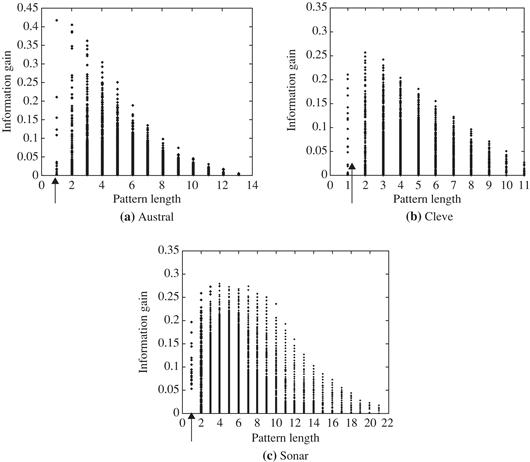
Figure 9.11 Single feature versus frequent pattern: Information gain is plotted for single features (patterns of length 1, indicated by arrows) and frequent patterns (combined features) for three UCI data sets. Source: Adapted from Cheng, Yan, Han, and Hsu [CYHH07].
“Why not consider frequent patterns as combined features, in addition to single features when building a classification model?” This notion is the basis of frequent pattern–based classification —the learning of a classification model in the feature space of single attributes as well as frequent patterns. In this way, we transfer the original feature space to a larger space. This will likely increase the chance of including important features.
Let’s get back to our earlier question: How discriminative are frequent patterns? Many of the frequent patterns generated in frequent itemset mining are indiscriminative because they are based solely on support, without considering predictive power. That is, by definition, a pattern must satisfy a user-specified minimum support threshold, min_sup, to be considered frequent. For example, if min_sup, is, say, 5%, a pattern is frequent if it occurs in 5% of the data tuples. Consider Figure 9.12, which plots information gain versus pattern frequency (support) for three UCI data sets. A theoretical upper bound on information gain, which was derived analytically, is also plotted. The figure shows that the discriminative power (assessed here as information gain) of low-frequency patterns is bounded by a small value. This is due to the patterns' limited coverage of the data set. Similarly, the discriminative power of very high-frequency patterns is also bounded by a small value, which is due to their commonness in the data. The upper bound of information gain is a function of pattern frequency. The information gain upper bound increases monotonically with pattern frequency. These observations can be confirmed analytically. Patterns with medium-large supports (e.g., support = 300 in Figure 9.12a) may be discriminative or not. Thus, not every frequent pattern is useful.
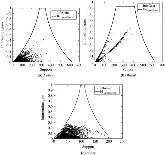
Figure 9.12 Information gain versus pattern frequency (support) for three UCI data sets. A theoretical upper bound on information gain (IGUpper Bound) is also shown. Source: Adapted from Cheng, Yan, Han, and Hsu [CYHH07].
If we were to add all the frequent patterns to the feature space, the resulting feature space would be huge. This slows down the model learning process and may also lead to decreased accuracy due to a form of overfitting in which there are too many features. Many of the patterns may be redundant. Therefore, it’s a good idea to apply feature selection to eliminate the less discriminative and redundant frequent patterns as features. The general framework for discriminative frequent pattern–based classification is as follows.
1. Feature generation: The data, D, are partitioned according to class label. Use frequent itemset mining to discover frequent patterns in each partition, satisfying minimum support. The collection of frequent patterns, ![]() , makes up the feature candidates.
, makes up the feature candidates.
2. Feature selection: Apply feature selection to ![]() , resulting in
, resulting in ![]() , the set of selected (more discriminating) frequent patterns. Information gain, Fisher score, or other evaluation measures can be used for this step. Relevancy checking can also be incorporated into this step to weed out redundant patterns. The data set D is transformed to
, the set of selected (more discriminating) frequent patterns. Information gain, Fisher score, or other evaluation measures can be used for this step. Relevancy checking can also be incorporated into this step to weed out redundant patterns. The data set D is transformed to ![]() , where the feature space now includes the single features as well as the selected frequent patterns,
, where the feature space now includes the single features as well as the selected frequent patterns, ![]() .
.
3. Learning of classification model: A classifier is built on the data set ![]() . Any learning algorithm can be used as the classification model.
. Any learning algorithm can be used as the classification model.
The general framework is summarized in Figure 9.13(a), where the discriminative patterns are represented by dark circles. Although the approach is straightforward, we can encounter a computational bottleneck by having to first find all the frequent patterns, and then analyze each one for selection. The amount of frequent patterns found can be huge due to the explosive number of pattern combinations between items.

Figure 9.13 A framework for frequent pattern–based classification: (a) a two-step general approach versus (b) the direct approach of DDPMine.
To improve the efficiency of the general framework, consider condensing steps 1 and 2 into just one step. That is, rather than generating the complete set of frequent patterns, it’s possible to mine only the highly discriminative ones. This more direct approach is referred to as direct discriminative pattern mining. The DDPMine algorithm follows this approach, as illustrated in Figure 9.13(b). It first transforms the training data into a compact tree structure known as a frequent pattern tree, or FP-tree (Section 6.2.4), which holds all of the attribute–value (itemset) association information. It then searches for discriminative patterns on the tree. The approach is direct in that it avoids generating a large number of indiscriminative patterns. It incrementally reduces the problem by eliminating training tuples, thereby progressively shrinking the FP-tree. This further speeds up the mining process.
By choosing to transform the original data to an FP-tree, DDPMine avoids generating redundant patterns because an FP-tree stores only the closed frequent patterns. By definition, any subpattern, β, of a closed pattern, α, is redundant with respect to α (Section 6.1.2). DDPMine directly mines the discriminative patterns and integrates feature selection into the mining framework. The theoretical upper bound on information gain is used to facilitate a branch-and-bound search, which prunes the search space significantly. Experimental results show that DDPMine achieves orders of magnitude speedup over the two-step approach without decline in classification accuracy. DDPMine also outperforms state-of-the-art associative classification methods in terms of both accuracy and efficiency.