
10.5 Grid-Based Methods
The clustering methods discussed so far are data-driven—they partition the set of objects and adapt to the distribution of the objects in the embedding space. Alternatively, a grid-based clustering method takes a space-driven approach by partitioning the embedding space into cells independent of the distribution of the input objects.
The grid-based clustering approach uses a multiresolution grid data structure. It quantizes the object space into a finite number of cells that form a grid structure on which all of the operations for clustering are performed. The main advantage of the approach is its fast processing time, which is typically independent of the number of data objects, yet dependent on only the number of cells in each dimension in the quantized space.
In this section, we illustrate grid-based clustering using two typical examples. STING (Section 10.5.1) explores statistical information stored in the grid cells. CLIQUE (Section 10.5.2) represents a grid- and density-based approach for subspace clustering in a high-dimensional data space.
10.5.1 STING: STatistical INformation Grid
STING is a grid-based multiresolution clustering technique in which the embedding spatial area of the input objects is divided into rectangular cells. The space can be divided in a hierarchical and recursive way. Several levels of such rectangular cells correspond to different levels of resolution and form a hierarchical structure: Each cell at a high level is partitioned to form a number of cells at the next lower level. Statistical information regarding the attributes in each grid cell, such as the mean, maximum, and minimum values, is precomputed and stored as statistical parameters. These statistical parameters are useful for query processing and for other data analysis tasks.
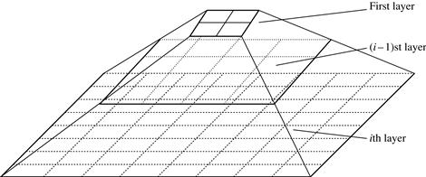
Figure 10.19 shows a hierarchical structure for STING clustering. The statistical parameters of higher-level cells can easily be computed from the parameters of the lower-level cells. These parameters include the following: the attribute-independent parameter, count; and the attribute-dependent parameters, mean, stdev (standard deviation), min (minimum), max (maximum), and the type of distribution that the attribute value in the cell follows such as normal, uniform, exponential, or none (if the distribution is unknown). Here, the attribute is a selected measure for analysis such as price for house objects. When the data are loaded into the database, the parameters count, mean, stdev, min, and max of the bottom-level cells are calculated directly from the data. The value of distribution may either be assigned by the user if the distribution type is known beforehand or obtained by hypothesis tests such as the χ2 test. The type of distribution of a higher-level cell can be computed based on the majority of distribution types of its corresponding lower-level cells in conjunction with a threshold filtering process. If the distributions of the lower-level cells disagree with each other and fail the threshold test, the distribution type of the high-level cell is set to none.
“How is this statistical information useful for query answering?” The statistical parameters can be used in a top-down, grid-based manner as follows. First, a layer within the hierarchical structure is determined from which the query-answering process is to start. This layer typically contains a small number of cells. For each cell in the current layer, we compute the confidence interval (or estimated probability range) reflecting the cell’s relevancy to the given query. The irrelevant cells are removed from further consideration. Processing of the next lower level examines only the remaining relevant cells. This process is repeated until the bottom layer is reached. At this time, if the query specification is met, the regions of relevant cells that satisfy the query are returned. Otherwise, the data that fall into the relevant cells are retrieved and further processed until they meet the query’s requirements.
An interesting property of STING is that it approaches the clustering result of DBSCAN if the granularity approaches 0 (i.e., toward very low-level data). In other words, using the count and cell size information, dense clusters can be identified approximately using STING. Therefore, STING can also be regarded as a density-based clustering method.
“What advantages does STING offer over other clustering methods?” STING offers several advantages: (1) the grid-based computation is query-independent because the statistical information stored in each cell represents the summary information of the data in the grid cell, independent of the query; (2) the grid structure facilitates parallel processing and incremental updating; and (3) the method’s efficiency is a major advantage: STING goes through the database once to compute the statistical parameters of the cells, and hence the time complexity of generating clusters is O(n), where n is the total number of objects. After generating the hierarchical structure, the query processing time is O(g), where g is the total number of grid cells at the lowest level, which is usually much smaller than n.
Because STING uses a multiresolution approach to cluster analysis, the quality of STING clustering depends on the granularity of the lowest level of the grid structure. If the granularity is very fine, the cost of processing will increase substantially; however, if the bottom level of the grid structure is too coarse, it may reduce the quality of cluster analysis. Moreover, STING does not consider the spatial relationship between the children and their neighboring cells for construction of a parent cell. As a result, the shapes of the resulting clusters are isothetic, that is, all the cluster boundaries are either horizontal or vertical, and no diagonal boundary is detected. This may lower the quality and accuracy of the clusters despite the fast processing time of the technique.
10.5.2 CLIQUE: An Apriori-like Subspace Clustering Method
A data object often has tens of attributes, many of which may be irrelevant. The values of attributes may vary considerably. These factors can make it difficult to locate clusters that span the entire data space. It may be more meaningful to instead search for clusters within different subspaces of the data. For example, consider a health-informatics application where patient records contain extensive attributes describing personal information, numerous symptoms, conditions, and family history.
Finding a nontrivial group of patients for which all or even most of the attributes strongly agree is unlikely. In bird flu patients, for instance, the age, gender, and job attributes may vary dramatically within a wide range of values. Thus, it can be difficult to find such a cluster within the entire data space. Instead, by searching in subspaces, we may find a cluster of similar patients in a lower-dimensional space (e.g., patients who are similar to one other with respect to symptoms like high fever, cough but no runny nose, and aged between 3 and 16).
CLIQUE (CLustering In QUEst) is a simple grid-based method for finding density-based clusters in subspaces. CLIQUE partitions each dimension into nonoverlapping intervals, thereby partitioning the entire embedding space of the data objects into cells. It uses a density threshold to identify dense cells and sparse ones. A cell is dense if the number of objects mapped to it exceeds the density threshold.
The main strategy behind CLIQUE for identifying a candidate search space uses the monotonicity of dense cells with respect to dimensionality. This is based on the Apriori property used in frequent pattern and association rule mining (Chapter 6). In the context of clusters in subspaces, the monotonicity says the following. A k-dimensional cell c(k > 1) can have at least l points only if every (k − 1)-dimensional projection of c, which is a cell in a (k − 1)-dimensional subspace, has at least l points. Consider Figure 10.20, where the embedding data space contains three dimensions: age, salary, and vacation. A 2-D cell, say in the subspace formed by age and salary, contains l points only if the projection of this cell in every dimension, that is, age and salary, respectively, contains at least l points.
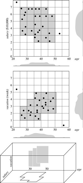
Figure 10.20 Dense units found with respect to age for the dimensions salary and vacation are intersected to provide a candidate search space for dense units of higher dimensionality.
CLIQUE performs clustering in two steps. In the first step, CLIQUE partitions the d-dimensional data space into nonoverlapping rectangular units, identifying the dense units among these. CLIQUE finds dense cells in all of the subspaces. To do so, CLIQUE partitions every dimension into intervals, and identifies intervals containing at least l points, where l is the density threshold. CLIQUE then iteratively joins two k-dimensional dense cells, c1 and c2, in subspaces (Di1, …, Dik) and (Dj1, …, Djk), respectively, if Di1 = Dj1, …, Dik − 1 = Djk − 1, and c1 and c2 share the same intervals in those dimensions. The join operation generates a new (k + 1)-dimensional candidate cell c in space (Di1, …, Dik − 1, Dik, Djk). CLIQUE checks whether the number of points in c passes the density threshold. The iteration terminates when no candidates can be generated or no candidate cells are dense.
In the second step, CLIQUE uses the dense cells in each subspace to assemble clusters, which can be of arbitrary shape. The idea is to apply the Minimum Description Length (MDL) principle (Chapter 8) to use the maximal regions to cover connected dense cells, where a maximal region is a hyperrectangle where every cell falling into this region is dense, and the region cannot be extended further in any dimension in the subspace. Finding the best description of a cluster in general is NP-Hard. Thus, CLIQUE adopts a simple greedy approach. It starts with an arbitrary dense cell, finds a maximal region covering the cell, and then works on the remaining dense cells that have not yet been covered. The greedy method terminates when all dense cells are covered.
“How effective is CLIQUE?” CLIQUE automatically finds subspaces of the highest dimensionality such that high-density clusters exist in those subspaces. It is insensitive to the order of input objects and does not presume any canonical data distribution. It scales linearly with the size of the input and has good scalability as the number of dimensions in the data is increased. However, obtaining a meaningful clustering is dependent on proper tuning of the grid size (which is a stable structure here) and the density threshold. This can be difficult in practice because the grid size and density threshold are used across all combinations of dimensions in the data set. Thus, the accuracy of the clustering results may be degraded at the expense of the method’s simplicity. Moreover, for a given dense region, all projections of the region onto lower-dimensionality subspaces will also be dense. This can result in a large overlap among the reported dense regions. Furthermore, it is difficult to find clusters of rather different densities within different dimensional subspaces.
Several extensions to this approach follow a similar philosophy. For example, we can think of a grid as a set of fixed bins. Instead of using fixed bins for each of the dimensions, we can use an adaptive, data-driven strategy to dynamically determine the bins for each dimension based on data distribution statistics. Alternatively, instead of using a density threshold, we may use entropy (Chapter 8) as a measure of the quality of subspace clusters.