
9.2 Classification by Backpropagation
“What is backpropagation?“ Backpropagation is a neural network learning algorithm. The neural networks field was originally kindled by psychologists and neurobiologists who sought to develop and test computational analogs of neurons. Roughly speaking, a neural network is a set of connected input/output units in which each connection has a weight associated with it. During the learning phase, the network learns by adjusting the weights so as to be able to predict the correct class label of the input tuples. Neural network learning is also referred to as connectionist learning due to the connections between units.
Neural networks involve long training times and are therefore more suitable for applications where this is feasible. They require a number of parameters that are typically best determined empirically such as the network topology or “structure." Neural networks have been criticized for their poor interpretability. For example, it is difficult for humans to interpret the symbolic meaning behind the learned weights and of “hidden units” in the network. These features initially made neural networks less desirable for data mining.
Advantages of neural networks, however, include their high tolerance of noisy data as well as their ability to classify patterns on which they have not been trained. They can be used when you may have little knowledge of the relationships between attributes and classes. They are well suited for continuous-valued inputs and outputs, unlike most decision tree algorithms. They have been successful on a wide array of real-world data, including handwritten character recognition, pathology and laboratory medicine, and training a computer to pronounce English text. Neural network algorithms are inherently parallel; parallelization techniques can be used to speed up the computation process. In addition, several techniques have been recently developed for rule extraction from trained neural networks. These factors contribute to the usefulness of neural networks for classification and numeric prediction in data mining.
There are many different kinds of neural networks and neural network algorithms. The most popular neural network algorithm is backpropagation, which gained repute in the 1980s. In Section 9.2.1 you will learn about multilayer feed-forward networks, the type of neural network on which the backpropagation algorithm performs. Section 9.2.2 discusses defining a network topology. The backpropagation algorithm is described in Section 9.2.3. Rule extraction from trained neural networks is discussed in Section 9.2.4.
9.2.1 A Multilayer Feed-Forward Neural Network
The backpropagation algorithm performs learning on a multilayer feed-forward neural network. It iteratively learns a set of weights for prediction of the class label of tuples. A multilayer feed-forward neural network consists of an input layer, one or more hidden layers, and an output layer. An example of a multilayer feed-forward network is shown in Figure 9.2.
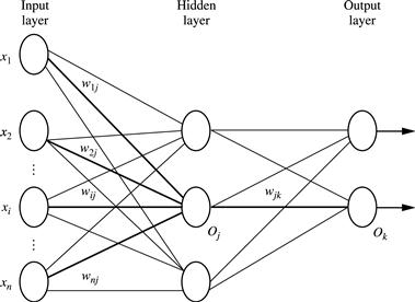
Each layer is made up of units. The inputs to the network correspond to the attributes measured for each training tuple. The inputs are fed simultaneously into the units making up the input layer. These inputs pass through the input layer and are then weighted and fed simultaneously to a second layer of “neuronlike” units, known as a hidden layer. The outputs of the hidden layer units can be input to another hidden layer, and so on. The number of hidden layers is arbitrary, although in practice, usually only one is used. The weighted outputs of the last hidden layer are input to units making up the output layer, which emits the network’s prediction for given tuples.
The units in the input layer are called input units. The units in the hidden layers and output layer are sometimes referred to as neurodes, due to their symbolic biological basis, or as output units. The multilayer neural network shown in Figure 9.2 has two layers of output units. Therefore, we say that it is a two-layer neural network. (The input layer is not counted because it serves only to pass the input values to the next layer.) Similarly, a network containing two hidden layers is called a three-layer neural network, and so on. It is a feed-forward network since none of the weights cycles back to an input unit or to a previous layer’s output unit. It is fully connected in that each unit provides input to each unit in the next forward layer.
Each output unit takes, as input, a weighted sum of the outputs from units in the previous layer (see Figure 9.4 later). It applies a nonlinear (activation) function to the weighted input. Multilayer feed-forward neural networks are able to model the class prediction as a nonlinear combination of the inputs. From a statistical point of view, they perform nonlinear regression. Multilayer feed-forward networks, given enough hidden units and enough training samples, can closely approximate any function.
9.2.2 Defining a Network Topology
“How can I design the neural network’s topology?” Before training can begin, the user must decide on the network topology by specifying the number of units in the input layer, the number of hidden layers (if more than one), the number of units in each hidden layer, and the number of units in the output layer.
Normalizing the input values for each attribute measured in the training tuples will help speed up the learning phase. Typically, input values are normalized so as to fall between 0.0 and 1.0. Discrete-valued attributes may be encoded such that there is one input unit per domain value. For example, if an attribute A has three possible or known values, namely ![]() , then we may assign three input units to represent A. That is, we may have, say,
, then we may assign three input units to represent A. That is, we may have, say, ![]() as input units. Each unit is initialized to 0. If
as input units. Each unit is initialized to 0. If ![]() , then I0 is set to 1 and the rest are 0. If
, then I0 is set to 1 and the rest are 0. If ![]() , then I1 is set to 1 and the rest are 0, and so on.
, then I1 is set to 1 and the rest are 0, and so on.
Neural networks can be used for both classification (to predict the class label of a given tuple) and numeric prediction (to predict a continuous-valued output). For classification, one output unit may be used to represent two classes (where the value 1 represents one class, and the value 0 represents the other). If there are more than two classes, then one output unit per class is used. (See Section 9.7.1 for more strategies on multiclass classification.)
There are no clear rules as to the “best” number of hidden layer units. Network design is a trial-and-error process and may affect the accuracy of the resulting trained network. The initial values of the weights may also affect the resulting accuracy. Once a network has been trained and its accuracy is not considered acceptable, it is common to repeat the training process with a different network topology or a different set of initial weights. Cross-validation techniques for accuracy estimation (described in Chapter 8) can be used to help decide when an acceptable network has been found. A number of automated techniques have been proposed that search for a “good” network structure. These typically use a hill-climbing approach that starts with an initial structure that is selectively modified.
9.2.3 Backpropagation
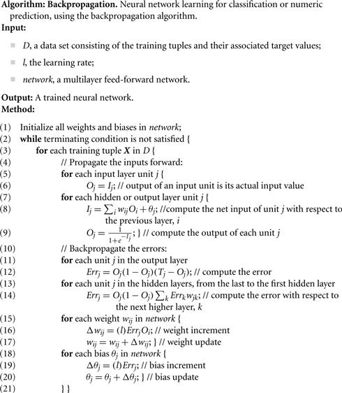
“How does backpropagation work?” Backpropagation learns by iteratively processing a data set of training tuples, comparing the network’s prediction for each tuple with the actual known target value. The target value may be the known class label of the training tuple (for classification problems) or a continuous value (for numeric prediction). For each training tuple, the weights are modified so as to minimize the mean-squared error between the network’s prediction and the actual target value. These modifications are made in the “backwards” direction (i.e., from the output layer) through each hidden layer down to the first hidden layer (hence the name backpropagation). Although it is not guaranteed, in general the weights will eventually converge, and the learning process stops. The algorithm is summarized in Figure 9.3. The steps involved are expressed in terms of inputs, outputs, and errors, and may seem awkward if this is your first look at neural network learning. However, once you become familiar with the process, you will see that each step is inherently simple. The steps are described next.
Initialize the weights: The weights in the network are initialized to small random numbers (e.g., ranging from −1.0 to 1.0, or −0.5 to 0.5). Each unit has a bias associated with it, as explained later. The biases are similarly initialized to small random numbers.
Each training tuple, X, is processed by the following steps.
Propagate the inputs forward: First, the training tuple is fed to the network’s input layer. The inputs pass through the input units, unchanged. That is, for an input unit, j, its output, Oj, is equal to its input value, Ij. Next, the net input and output of each unit in the hidden and output layers are computed. The net input to a unit in the hidden or output layers is computed as a linear combination of its inputs. To help illustrate this point, a hidden layer or output layer unit is shown in Figure 9.4. Each such unit has a number of inputs to it that are, in fact, the outputs of the units connected to it in the previous layer. Each connection has a weight. To compute the net input to the unit, each input connected to the unit is multiplied by its corresponding weight, and this is summed. Given a unit, j in a hidden or output layer, the net input, Ij, to unit j is
![]() (9.4)
(9.4)
where ![]() is the weight of the connection from unit i in the previous layer to unit j; Oi is the output of unit i from the previous layer; and
is the weight of the connection from unit i in the previous layer to unit j; Oi is the output of unit i from the previous layer; and ![]() is the bias of the unit. The bias acts as a threshold in that it serves to vary the activity of the unit.
is the bias of the unit. The bias acts as a threshold in that it serves to vary the activity of the unit.
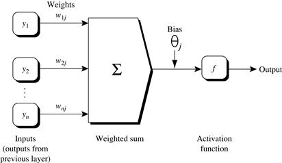
Figure 9.4 Hidden or output layer unit j: The inputs to unit j are outputs from the previous layer. These are multiplied by their corresponding weights to form a weighted sum, which is added to the bias associated with unit j. A nonlinear activation function is applied to the net input. (For ease of explanation, the inputs to unit j are labeled y1, y2,…,yn. If unit j were in the first hidden layer, then these inputs would correspond to the input tuple (x1, x2,…,xn).)
Each unit in the hidden and output layers takes its net input and then applies an activation function to it, as illustrated in Figure 9.4. The function symbolizes the activation of the neuron represented by the unit. The logistic, or sigmoid, function is used. Given the net input Ij to unit j, then Oj, the output of unit j, is computed as
![]() (9.5)
(9.5)
This function is also referred to as a squashing function, because it maps a large input domain onto the smaller range of 0 to 1. The logistic function is nonlinear and differentiable, allowing the backpropagation algorithm to model classification problems that are linearly inseparable.
We compute the output values, Oj, for each hidden layer, up to and including the output layer, which gives the network’s prediction. In practice, it is a good idea to cache (i.e., save) the intermediate output values at each unit as they are required again later when backpropagating the error. This trick can substantially reduce the amount of computation required.
Backpropagate the error: The error is propagated backward by updating the weights and biases to reflect the error of the network’s prediction. For a unit j in the output layer, the error Errj is computed by
![]() (9.6)
(9.6)
where Oj is the actual output of unit j, and Tj is the known target value of the given training tuple. Note that ![]() is the derivative of the logistic function.
is the derivative of the logistic function.
To compute the error of a hidden layer unit j, the weighted sum of the errors of the units connected to unit j in the next layer are considered. The error of a hidden layer unit j is
![]() (9.7)
(9.7)
where wjk is the weight of the connection from unit j to a unit k in the next higher layer, and Errk is the error of unit k.
The weights and biases are updated to reflect the propagated errors. Weights are updated by the following equations, where ![]() is the change in weight
is the change in weight ![]() :
:
![]() (9.8)
(9.8)
![]() (9.9)
(9.9)
“What is l in Eq. (9.8)?” The variable l is the learning rate, a constant typically having a value between 0.0 and 1.0. Backpropagation learns using a gradient descent method to search for a set of weights that fits the training data so as to minimize the mean-squared distance between the network’s class prediction and the known target value of the tuples.1 The learning rate helps avoid getting stuck at a local minimum in decision space (i.e., where the weights appear to converge, but are not the optimum solution) and encourages finding the global minimum. If the learning rate is too small, then learning will occur at a very slow pace. If the learning rate is too large, then oscillation between inadequate solutions may occur. A rule of thumb is to set the learning rate to 1/t, where t is the number of iterations through the training set so far.
Biases are updated by the following equations, where ![]() is the change in bias
is the change in bias ![]() :
:
![]() (9.10)
(9.10)
![]() (9.11)
(9.11)
Note that here we are updating the weights and biases after the presentation of each tuple. This is referred to as case updating. Alternatively, the weight and bias increments could be accumulated in variables, so that the weights and biases are updated after all the tuples in the training set have been presented. This latter strategy is called epoch updating, where one iteration through the training set is an epoch. In theory, the mathematical derivation of backpropagation employs epoch updating, yet in practice, case updating is more common because it tends to yield more accurate results.
Terminating condition: Training stops when
■ All ![]() in the previous epoch are so small as to be below some specified threshold, or
in the previous epoch are so small as to be below some specified threshold, or
■ The percentage of tuples misclassified in the previous epoch is below some threshold, or
In practice, several hundreds of thousands of epochs may be required before the weights will converge.
“How efficient is backpropagation?” The computational efficiency depends on the time spent training the network. Given ![]() tuples and w weights, each epoch requires
tuples and w weights, each epoch requires ![]() time. However, in the worst-case scenario, the number of epochs can be exponential in n, the number of inputs. In practice, the time required for the networks to converge is highly variable. A number of techniques exist that help speed up the training time. For example, a technique known as simulated annealing can be used, which also ensures convergence to a global optimum.
time. However, in the worst-case scenario, the number of epochs can be exponential in n, the number of inputs. In practice, the time required for the networks to converge is highly variable. A number of techniques exist that help speed up the training time. For example, a technique known as simulated annealing can be used, which also ensures convergence to a global optimum.
Example 9.1
Sample calculations for learning by the backpropagation algorithm
Figure 9.5 shows a multilayer feed-forward neural network. Let the learning rate be 0.9. The initial weight and bias values of the network are given in Table 9.1, along with the first training tuple, ![]() , with a class label of 1.
, with a class label of 1.
This example shows the calculations for backpropagation, given the first training tuple, X. The tuple is fed into the network, and the net input and output of each unit are computed. These values are shown in Table 9.2. The error of each unit is computed and propagated backward. The error values are shown in Table 9.3. The weight and bias updates are shown in Table 9.4.
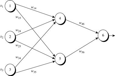
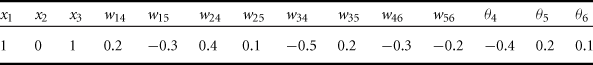
Table 9.2
Net Input and Output Calculations
| Unit, j | Net Input, Ij | Output, Oj |
| 4 | 0.2 + 0 − 0.5 − 0.4 = −0.7 | 1/(1 + e0.7) = 0.332 |
| 5 | −0.3 + 0 + 0.2 + 0.2 = 0.1 | 1/(1 + e−0.1) = 0.525 |
| 6 | (−0.3)(0.332) − (0.2)(0.525) + 0.1 = −0.105 | 1/(1 + e0.105) = 0.474 |
Table 9.3
Calculation of the Error at Each Node
| Unit, j | Errj |
| 6 | (0.474)(1 − 0.474)(1 − 0.474) = 0.1311 |
| 5 | (0.525)(1 − 0.525)(0.1311)(−0.2) = −0.0065 |
| 4 | (0.332)(1 − 0.332)(0.1311)(−0.3) = −0.0087 |
Table 9.4
Calculations for Weight and Bias Updating
| Weight or Bias | New Value |
| w46 | −0.3 + (0.9)(0.1311)(0.332) = −0.261 |
| w56 | −0.2 + (0.9)(0.1311)(0.525) = −0.138 |
| w14 | 0.2 + (0.9)(−0.0087)(1) = 0.192 |
| w15 | −0.3 + (0.9)(−0.0065)(1) = −0.306 |
| w24 | 0.4 + (0.9)(−0.0087)(0) = 0.4 |
| w25 | 0.1 + (0.9)(−0.0065)(0) = 0.1 |
| w34 | −0.5 + (0.9)(−0.0087)(1) = −0.508 |
| w35 | 0.2 + (0.9)(−0.0065)(1) = 0.194 |
| θ6 | 0.1 + (0.9)(0.1311) = 0.218 |
| θ5 | 0.2 + (0.9)(−0.0065) = 0.194 |
| θ4 | −0.4 + (0.9)(−0.0087) = −0.408 |
“How can we classify an unknown tuple using a trained network?” To classify an unknown tuple, X, the tuple is input to the trained network, and the net input and output of each unit are computed. (There is no need for computation and/or backpropagation of the error.) If there is one output node per class, then the output node with the highest value determines the predicted class label for X. If there is only one output node, then output values greater than or equal to 0.5 may be considered as belonging to the positive class, while values less than 0.5 may be considered negative.
Several variations and alternatives to the backpropagation algorithm have been proposed for classification in neural networks. These may involve the dynamic adjustment of the network topology and of the learning rate or other parameters, or the use of different error functions.
9.2.4 Inside the Black Box: Backpropagation and Interpretability
“Neural networks are like a black box. How can I 'understand' what the backpropagation network has learned?” A major disadvantage of neural networks lies in their knowledge representation. Acquired knowledge in the form of a network of units connected by weighted links is difficult for humans to interpret. This factor has motivated research in extracting the knowledge embedded in trained neural networks and in representing that knowledge symbolically. Methods include extracting rules from networks and sensitivity analysis.
Various algorithms for rule extraction have been proposed. The methods typically impose restrictions regarding procedures used in training the given neural network, the network topology, and the discretization of input values.
Fully connected networks are difficult to articulate. Hence, often the first step in extracting rules from neural networks is network pruning. This consists of simplifying the network structure by removing weighted links that have the least effect on the trained network. For example, a weighted link may be deleted if such removal does not result in a decrease in the classification accuracy of the network.
Once the trained network has been pruned, some approaches will then perform link, unit, or activation value clustering. In one method, for example, clustering is used to find the set of common activation values for each hidden unit in a given trained two-layer neural network (Figure 9.6). The combinations of these activation values for each hidden unit are analyzed. Rules are derived relating combinations of activation values with corresponding output unit values. Similarly, the sets of input values and activation values are studied to derive rules describing the relationship between the input layer and the hidden “layer units”? Finally, the two sets of rules may be combined to form IF-THEN rules. Other algorithms may derive rules of other forms, including M-of-N rules (where M out of a given N conditions in the rule antecedent must be true for the rule consequent to be applied), decision trees with M-of-N tests, fuzzy rules, and finite automata.
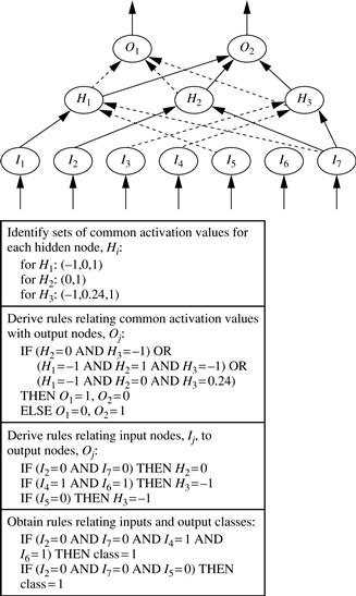
Figure 9.6 Rules can be extracted from training neural networks. Source: Adapted from Lu, Setiono, and Liu [LSL95].
Sensitivity analysis is used to assess the impact that a given input variable has on a network output. The input to the variable is varied while the remaining input variables are fixed at some value. Meanwhile, changes in the network output are monitored. The knowledge gained from this analysis form can be represented in rules such as “IF X decreases 5% THEN Y increases 8%.”