
9.7 Additional Topics Regarding Classification
Most of the classification algorithms we have studied handle multiple classes, but some, such as support vector machines, assume only two classes exist in the data. What adaptations can be made to allow for when there are more than two classes? This question is addressed in Section 9.7.1 on multiclass classification.
What can we do if we want to build a classifier for data where only some of the data are class-labeled, but most are not? Document classification, speech recognition, and information extraction are just a few examples of applications in which unlabeled data are abundant. Consider document classification, for example. Suppose we want to build a model to automatically classify text documents like articles or web pages. In particular, we want the model to distinguish between hockey and football documents. We have a vast amount of documents available, yet the documents are not class-labeled. Recall that supervised learning requires a training set, that is, a set of classlabeled data. To have a human examine and assign a class label to individual documents (to form a training set) is time consuming and expensive.
Speech recognition requires the accurate labeling of speech utterances by trained linguists. It was reported that 1 minute of speech takes 10 minutes to label, and annotating phonemes (basic units of sound) can take 400 times as long. Information extraction systems are trained using labeled documents with detailed annotations. These are obtained by having human experts highlight items or relations of interest in text such as the names of companies or individuals. High-level expertise may be required for certain knowledge domains such as gene and disease mentions in biomedical information extraction. Clearly, the manual assignment of class labels to prepare a training set can be extremely costly, time consuming, and tedious.
We study three approaches to classification that are suitable for situations where there is an abundance of unlabeled data. Section 9.7.2 introduces semisupervised classification, which builds a classifier using both labeled and unlabeled data. Section 9.7.3 presents active learning, where the learning algorithm carefully selects a few of the unlabeled data tuples and asks a human to label only those tuples. Section 9.7.4 presents transfer learning, which aims to extract the knowledge from one or more source tasks (e.g., classifying camera reviews) and apply the knowledge to a target task (e.g., TV reviews). Each of these strategies can reduce the need to annotate large amounts of data, resulting in cost and time savings.
9.7.1 Multiclass Classification
Some classification algorithms, such as support vector machines, are designed for binary classification. How can we extend these algorithms to allow for multiclass classification (i.e., classification involving more than two classes)?
A simple approach is one-versus-all (OVA). Given m classes, we train m binary classifiers, one for each class. Classifier j is trained using tuples of class j as the positive class, and the remaining tuples as the negative class. It learns to return a positive value for class j and a negative value for the rest. To classify an unknown tuple, X, the set of classifiers vote as an ensemble. For example, if classifier j predicts the positive class for X, then class j gets one vote. If it predicts the negative class for X, then each of the classes except j gets one vote. The class with the most votes is assigned to X.
All-versus-all (AVA) is an alternative approach that learns a classifier for each pair of classes. Given m classes, we construct ![]() binary classifiers. A classifier is trained using tuples of the two classes it should discriminate. To classify an unknown tuple, each classifier votes. The tuple is assigned the class with the maximum number of votes. All-versus-all tends to be superior to one-versus-all.
binary classifiers. A classifier is trained using tuples of the two classes it should discriminate. To classify an unknown tuple, each classifier votes. The tuple is assigned the class with the maximum number of votes. All-versus-all tends to be superior to one-versus-all.
A problem with the previous schemes is that binary classifiers are sensitive to errors. If any classifier makes an error, it can affect the vote count.
Error-correcting codes can be used to improve the accuracy of multiclass classification, not just in the previous situations, but for classification in general. Error-correcting codes were originally designed to correct errors during data transmission for communication tasks. For such tasks, the codes are used to add redundancy to the data being transmitted so that, even if some errors occur due to noise in the channel, the data can be correctly received at the other end. For multiclass classification, even if some of the individual binary classifiers make a prediction error for a given unknown tuple, we may still be able to correctly label the tuple.
An error-correcting code is assigned to each class, where each code is a bit vector. Figure 9.16 show an example of 7-bit codewords assigned to classes ![]() , and C4. We train one classifier for each bit position. Therefore, in our example we train seven classifiers. If a classifier makes an error, there is a better chance that we may still be able to predict the right class for a given unknown tuple because of the redundancy gained by having additional bits. The technique uses a distance measurement called the Hamming distance to guess the “closest” class in case of errors, and is illustrated in Example 9.3.
, and C4. We train one classifier for each bit position. Therefore, in our example we train seven classifiers. If a classifier makes an error, there is a better chance that we may still be able to predict the right class for a given unknown tuple because of the redundancy gained by having additional bits. The technique uses a distance measurement called the Hamming distance to guess the “closest” class in case of errors, and is illustrated in Example 9.3.
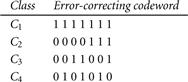
Error-correcting codes can correct up to ![]() 1-bit errors, where h is the minimum Hamming distance between any two codewords. If we use one bit per class, such as for 4-bit codewords for classes C1 through C4, then this is equivalent to the one-versus-all approach, and the codes are not sufficient to self-correct. (Try it as an exercise.) When selecting error-correcting codes for multiclass classification, there must be good row-wise and column-wise separation between the codewords. The greater the distance, the more likely that errors will be corrected.
1-bit errors, where h is the minimum Hamming distance between any two codewords. If we use one bit per class, such as for 4-bit codewords for classes C1 through C4, then this is equivalent to the one-versus-all approach, and the codes are not sufficient to self-correct. (Try it as an exercise.) When selecting error-correcting codes for multiclass classification, there must be good row-wise and column-wise separation between the codewords. The greater the distance, the more likely that errors will be corrected.
9.7.2 Semi-Supervised Classification
Semi-supervised classification uses labeled data and unlabeled data to build a classifier. Let ![]() be the set of labeled data and
be the set of labeled data and ![]() be the set of unlabeled data. Here we describe a few examples of this approach for learning.
be the set of unlabeled data. Here we describe a few examples of this approach for learning.
Self-training is the simplest form of semi-supervised classification. It first builds a classifier using the labeled data. The classifier then tries to label the unlabeled data. The tuple with the most confident label prediction is added to the set of labeled data, and the process repeats (Figure 9.17). Although the method is easy to understand, a disadvantage is that it may reinforce errors.
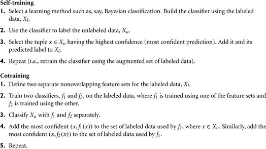
Cotraining is another form of semi-supervised classification, where two or more classifiers teach each other. Each learner uses a different and ideally independent set of features for each tuple. Consider web page data, for example, where attributes relating to the images on the page may be used as one set of features, while attributes relating to the corresponding text constitute another set of features for the same data. Each set of features should be sufficient to train a good classifier. Suppose we split the feature set into two sets and train two classifiers, f1 and f2, where each classifier is trained on a different set. Then, f1 and f2 are used to predict the class labels for the unlabeled data, Xu. Each classifier then teaches the other in that the tuple having the most confident prediction from f1 is added to the set of labeled data for f2 (along with its label).
Similarly, the tuple having the most confident prediction from f2 is added to the set of labeled data for f1. The method is summarized in Figure 9.17. Cotraining is less sensitive to errors than self-training. A difficulty is that the assumptions for its usage may not hold true, that is, it may not be possible to split the features into mutually exclusive and class-conditionally independent sets.
Alternate approaches to semi-supervised learning exist. For example, we can model the joint probability distribution of the features and the labels. For the unlabeled data, the labels can then be treated as missing data. The EM algorithm (Chapter 11) can be used to maximize the likelihood of the model. Methods using support vector machines have also been proposed.
9.7.3 Active Learning
Active learning is an iterative type of supervised learning that is suitable for situations where data are abundant, yet the class labels are scarce or expensive to obtain. The learning algorithm is active in that it can purposefully query a user (e.g., a human oracle) for labels. The number of tuples used to learn a concept this way is often much smaller than the number required in typical supervised learning.
“How does active learning work to overcome the labeling bottleneck?” To keep costs down, the active learner aims to achieve high accuracy using as few labeled instances as possible. Let D be all of data under consideration. Various strategies exist for active learning on D. Figure 9.18 illustrates a pool-based approach to active learning. Suppose that a small subset of D is class-labeled. This set is denoted L. U is the set of unlabeled data in D. It is also referred to as a pool of unlabeled data. An active learner begins with L as the initial training set. It then uses a querying function to carefully select one or more data samples from U and requests labels for them from an oracle (e.g., a human annotator). The newly labeled samples are added to L, which the learner then uses in a standard supervised way. The process repeats. The active learning goal is to achieve high accuracy using as few labeled tuples as possible. Active learning algorithms are typically evaluated with the use of learning curves, which plot accuracy as a function of the number of instances queried.
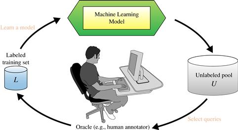
Figure 9.18 The pool-based active learning cycle. Source: From Settles [Set10], Burr Settles Computer Sciences Technical Report 1648, University of Wisconsin–Madison; used with permission.
Most of the active learning research focuses on how to choose the data tuples to be queried. Several frameworks have been proposed. Uncertainty sampling is the most common, where the active learner chooses to query the tuples which it is the least certain how to label. Other strategies work to reduce the version space, that is, the subset of all hypotheses that are consistent with the observed training tuples. Alternatively, we may follow a decision-theoretic approach that estimates expected error reduction. This selects tuples that would result in the greatest reduction in the total number of incorrect predictions such as by reducing the expected entropy over U. This latter approach tends to be more computationally expensive.
9.7.4 Transfer Learning
Suppose that AllElectronics has collected a number of customer reviews on a product such as a brand of camera. The classification task is to automatically label the reviews as either positive or negative. This task is known as sentiment classification. We could examine each review and annotate it by adding a positive or negative class label. The labeled reviews can then be used to train and test a classifier to label future reviews of the product as either positive or negative. The manual effort involved in annotating the review data can be expensive and time consuming.
Suppose that AllElectronics has customer reviews for other products as well such as TVs. The distribution of review data for different types of products can vary greatly. We cannot assume that the TV-review data will have the same distribution as the camera-review data; thus we must build a separate classification model for the TV-review data. Examining and labeling the TV-review data to form a training set will require a lot of effort. In fact, we would need to label a large amount of the data to train the review-classification models for each product. It would be nice if we could adapt an existing classification model (e.g., the one we built for cameras) to help learn a classification model for TVs. Such knowledge transfer would reduce the need to annotate a large amount of data, resulting in cost and time savings. This is the essence behind transfer learning.
Transfer learning aims to extract the knowledge from one or more source tasks and apply the knowledge to a target task. In our example, the source task is the classification of camera reviews, and the target task is the classification of TV reviews. Figure 9.19 illustrates a comparison between traditional learning methods and transfer learning. Traditional learning methods build a new classifier for each new classification task, based on available class-labeled training and test data. Transfer learning algorithms apply knowledge about source tasks when building a classifier for a new (target) task. Construction of the resulting classifier requires fewer training data and less training time. Traditional learning algorithms assume that the training data and test data are drawn from the same distribution and the same feature space. Thus, if the distribution changes, such methods need to rebuild the models from scratch.
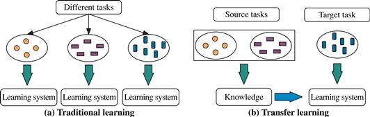
Figure 9.19 Transfer learning versus traditional learning. (a) Traditional learning methods build a new classifier from scratch for each classification task. (b) Transfer learning applies knowledge from a source classifier to simplify the construction of a classifier for a new, target task. Source: From Pan and Yang [PY10]; used with permission.
Transfer learning allows the distributions, tasks, and even the data domains used in training and testing to be different. Transfer learning is analogous to the way humans may apply their knowledge of a task to facilitate the learning of another task. For example, if we know how to play the recorder, we may apply our knowledge of note reading and music to simplify the task of learning to play the piano. Similarly, knowing Spanish may make it easier to learn Italian.
Transfer learning is useful for common applications where the data become outdated or the distribution changes. Here we give two more examples. Consider web-document classification, where we may have trained a classifier to label, say, articles from various newsgroups according to predefined categories. The web data that were used to train the classifier can easily become outdated because the topics on the Web change frequently. Another application area for transfer learning is email spam filtering. We could train a classifier to label email as either “spam” or “not spam,” using email from a group of users. If new users come along, the distribution of their email can be different from the original group, hence the need to adapt the learned model to incorporate the new data.
There are various approaches to transfer learning, the most common of which is the instance-based transfer learning approach. This approach reweights some of the data from the source task and uses it to learn the target task. The TrAdaBoost (Transfer AdaBoost) algorithm exemplifies this approach. Consider our previous example of web-document classification, where the distribution of the old data on which the classifier was trained (the source data) is different from the newer data (the target data). TrAdaBoost assumes that the source and target domain data are each described by the same set of attributes (i.e., they have the same “feature space”) and the same set of class labels, but that the distribution of the data in the two domains is very different. It extends the AdaBoost ensemble method described in Section 8.6.3. TrAdaBoost requires the labeling of only a small amount of the target data. Rather than throwing out all the old source data, TrAdaBoost assumes that a large amount of it can be useful in training the new classification model. The idea is to filter out the influence of any old data that are very different from the new data by automatically adjusting weights assigned to the training tuples.
Recall that in boosting, an ensemble is created by learning a series of classifiers. To begin, each tuple is assigned a weight. After a classifier Mi is learned, the weights are updated to allow the subsequent classifier, ![]() , to “pay more attention” to the training tuples that were misclassified by Mi. TrAdaBoost follows this strategy for the target data. However, if a source data tuple is misclassified, TrAdaBoost reasons that the tuple is probably very different from the target data. It therefore reduces the weight of such tuples so that they will have less effect on the subsequent classifier. As a result, TrAdaBoost can learn an accurate classification model using only a small amount of new data and a large amount of old data, even when the new data alone are insufficient to train the model. Hence, in this way TrAdaBoost allows knowledge to be transferred from the old classifier to the new one.
, to “pay more attention” to the training tuples that were misclassified by Mi. TrAdaBoost follows this strategy for the target data. However, if a source data tuple is misclassified, TrAdaBoost reasons that the tuple is probably very different from the target data. It therefore reduces the weight of such tuples so that they will have less effect on the subsequent classifier. As a result, TrAdaBoost can learn an accurate classification model using only a small amount of new data and a large amount of old data, even when the new data alone are insufficient to train the model. Hence, in this way TrAdaBoost allows knowledge to be transferred from the old classifier to the new one.
A challenge with transfer learning is negative transfer, which occurs when the new classifier performs worse than if there had been no transfer at all. Work on how to avoid negative transfer is an area of future research. Heterogeneous transfer learning, which involves transferring knowledge from different feature spaces and multiple source domains, is another venue for further work. Much of the research on transfer learning to date has been on small-scale applications. The use of transfer learning on larger applications, such as social network analysis and video classification, is an area for further investigation.