
9.3 Support Vector Machines
In this section, we study support vector machines (SVMs), a method for the classification of both linear and nonlinear data. In a nutshell, an SVM is an algorithm that works as follows. It uses a nonlinear mapping to transform the original training data into a higher dimension. Within this new dimension, it searches for the linear optimal separating hyperplane (i.e., a “decision boundary” separating the tuples of one class from another). With an appropriate nonlinear mapping to a sufficiently high dimension, data from two classes can always be separated by a hyperplane. The SVM finds this hyperplane using support vectors (“essential” training tuples) and margins (defined by the support vectors). We will delve more into these new concepts later.
“I’ve heard that SVMs have attracted a great deal of attention lately. Why?” The first paper on support vector machines was presented in 1992 by Vladimir Vapnik and colleagues Bernhard Boser and Isabelle Guyon, although the groundwork for SVMs has been around since the 1960s (including early work by Vapnik and Alexei Chervonenkis on statistical learning theory). Although the training time of even the fastest SVMs can be extremely slow, they are highly accurate, owing to their ability to model complex nonlinear decision boundaries. They are much less prone to overfitting than other methods. The support vectors found also provide a compact description of the learned model. SVMs can be used for numeric prediction as well as classification. They have been applied to a number of areas, including handwritten digit recognition, object recognition, and speaker identification, as well as benchmark time-series prediction tests.
9.3.1 The Case When the Data Are Linearly Separable
To explain the mystery of SVMs, let’s first look at the simplest case—a two-class problem where the classes are linearly separable. Let the data set D be given as (![]() , y1), (
, y1), (![]() , y2),…, (
, y2),…, (![]() ,
, ![]() ), where
), where ![]() is the set of training tuples with associated class labels, yi. Each yi can take one of two values, either +1 or −1 (i.e.,
is the set of training tuples with associated class labels, yi. Each yi can take one of two values, either +1 or −1 (i.e., ![]() ), corresponding to the classes buys_computer = yes and buys_computer = no, respectively. To aid in visualization, let’s consider an example based on two input attributes, A1 and A2, as shown in Figure 9.7. From the graph, we see that the 2-D data are linearly separable (or “linear," for short), because a straight line can be drawn to separate all the tuples of class +1 from all the tuples of class −1.
), corresponding to the classes buys_computer = yes and buys_computer = no, respectively. To aid in visualization, let’s consider an example based on two input attributes, A1 and A2, as shown in Figure 9.7. From the graph, we see that the 2-D data are linearly separable (or “linear," for short), because a straight line can be drawn to separate all the tuples of class +1 from all the tuples of class −1.
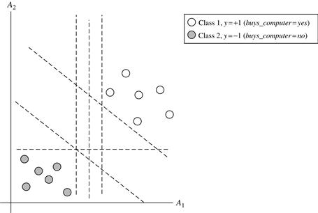
Figure 9.7 The 2-D training data are linearly separable. There are an infinite number of possible separating hyperplanes or “decision boundaries,” some of which are shown here as dashed lines. Which one is best?
There are an infinite number of separating lines that could be drawn. We want to find the “best” one, that is, one that (we hope) will have the minimum classification error on previously unseen tuples. How can we find this best line? Note that if our data were 3-D (i.e., with three attributes), we would want to find the best separating plane. Generalizing to n dimensions, we want to find the best hyperplane. We will use “hyperplane” to refer to the decision boundary that we are seeking, regardless of the number of input attributes. So, in other words, how can we find the best hyperplane?
An SVM approaches this problem by searching for the maximum marginal hyperplane. Consider Figure 9.8, which shows two possible separating hyperplanes and their associated margins. Before we get into the definition of margins, let’s take an intuitive look at this figure. Both hyperplanes can correctly classify all the given data tuples. Intuitively, however, we expect the hyperplane with the larger margin to be more accurate at classifying future data tuples than the hyperplane with the smaller margin. This is why (during the learning or training phase) the SVM searches for the hyperplane with the largest margin, that is, the maximum marginal hyperplane (MMH). The associated margin gives the largest separation between classes.
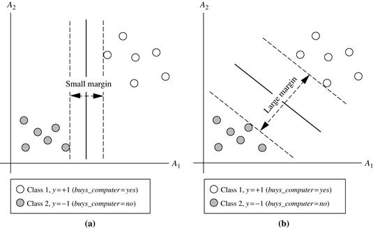
Figure 9.8 Here we see just two possible separating hyperplanes and their associated margins. Which one is better? The one with the larger margin (b) should have greater generalization accuracy.
Getting to an informal definition of margin, we can say that the shortest distance from a hyperplane to one side of its margin is equal to the shortest distance from the hyperplane to the other side of its margin, where the “sides” of the margin are parallel to the hyperplane. When dealing with the MMH, this distance is, in fact, the shortest distance from the MMH to the closest training tuple of either class.
A separating hyperplane can be written as
![]() (9.12)
(9.12)
where W is a weight vector, namely, ![]() ; n is the number of attributes; and b is a scalar, often referred to as a bias. To aid in visualization, let’s consider two input attributes, A1 and A2, as in Figure 9.8(b). Training tuples are 2-D (e.g.,
; n is the number of attributes; and b is a scalar, often referred to as a bias. To aid in visualization, let’s consider two input attributes, A1 and A2, as in Figure 9.8(b). Training tuples are 2-D (e.g., ![]() ), where x1 and x2 are the values of attributes A1 and A2, respectively, for X. If we think of b as an additional weight, w0, we can rewrite Eq. (9.12) as
), where x1 and x2 are the values of attributes A1 and A2, respectively, for X. If we think of b as an additional weight, w0, we can rewrite Eq. (9.12) as
![]() (9.13)
(9.13)
Thus, any point that lies above the separating hyperplane satisfies
![]() (9.14)
(9.14)
Similarly, any point that lies below the separating hyperplane satisfies
![]() (9.15)
(9.15)
The weights can be adjusted so that the hyperplanes defining the “sides” of the margin can be written as
![]() (9.16)
(9.16)
![]() (9.17)
(9.17)
That is, any tuple that falls on or above H1 belongs to class +1, and any tuple that falls on or below H2 belongs to class −1. Combining the two inequalities of Eqs. (9.16) and (9.17), we get
![]() (9.18)
(9.18)
Any training tuples that fall on hyperplanes H1 or H2 (i.e., the “sides” defining the margin) satisfy Eq. (9.18) and are called support vectors. That is, they are equally close to the (separating) MMH. In Figure 9.9, the support vectors are shown encircled with a thicker border. Essentially, the support vectors are the most difficult tuples to classify and give the most information regarding classification.

Figure 9.9 Support vectors. The SVM finds the maximum separating hyperplane, that is, the one with maximum distance between the nearest training tuples. The support vectors are shown with a thicker border.
From this, we can obtain a formula for the size of the maximal margin. The distance from the separating hyperplane to any point on H1 is ![]() , where
, where ![]() is the Euclidean norm of W, that is,
is the Euclidean norm of W, that is, ![]() .2 By definition, this is equal to the distance from any point on H2 to the separating hyperplane. Therefore, the maximal margin is
.2 By definition, this is equal to the distance from any point on H2 to the separating hyperplane. Therefore, the maximal margin is ![]() .
.
“So, how does an SVM find the MMH and the support vectors?” Using some “fancy math tricks," we can rewrite Eq. (9.18) so that it becomes what is known as a constrained (convex) quadratic optimization problem. Such fancy math tricks are beyond the scope of this book. Advanced readers may be interested to note that the tricks involve rewriting Eq. (9.18) using a Lagrangian formulation and then solving for the solution using Karush-Kuhn-Tucker (KKT) conditions. Details can be found in the bibliographic notes at the end of this chapter (Section 9.10).
If the data are small (say, less than 2000 training tuples), any optimization software package for solving constrained convex quadratic problems can then be used to find the support vectors and MMH. For larger data, special and more efficient algorithms for training SVMs can be used instead, the details of which exceed the scope of this book. Once we’ve found the support vectors and MMH (note that the support vectors define the MMH!), we have a trained support vector machine. The MMH is a linear class boundary, and so the corresponding SVM can be used to classify linearly separable data. We refer to such a trained SVM as a linear SVM.
“Once I’ve got a trained support vector machine, how do I use it to classify test (i.e., new) tuples?” Based on the Lagrangian formulation mentioned before, the MMH can be rewritten as the decision boundary
![]() (9.19)
(9.19)
where yi is the class label of support vector ![]() ;
; ![]() is a test tuple;
is a test tuple; ![]() and b0 are numeric parameters that were determined automatically by the optimization or SVM algorithm noted before; and l is the number of support vectors.
and b0 are numeric parameters that were determined automatically by the optimization or SVM algorithm noted before; and l is the number of support vectors.
Interested readers may note that the ![]() are Lagrangian multipliers. For linearly separable data, the support vectors are a subset of the actual training tuples (although there will be a slight twist regarding this when dealing with nonlinearly separable data, as we shall see in the following).
are Lagrangian multipliers. For linearly separable data, the support vectors are a subset of the actual training tuples (although there will be a slight twist regarding this when dealing with nonlinearly separable data, as we shall see in the following).
Given a test tuple, ![]() , we plug it into Eq. (9.19), and then check to see the sign of the result. This tells us on which side of the hyperplane the test tuple falls. If the sign is positive, then
, we plug it into Eq. (9.19), and then check to see the sign of the result. This tells us on which side of the hyperplane the test tuple falls. If the sign is positive, then ![]() falls on or above the MMH, and so the SVM predicts that
falls on or above the MMH, and so the SVM predicts that ![]() belongs to class +1 (representing buys_computer = yes, in our case). If the sign is negative, then
belongs to class +1 (representing buys_computer = yes, in our case). If the sign is negative, then ![]() falls on or below the MMH and the class prediction is −1 (representing buys_computer = no).
falls on or below the MMH and the class prediction is −1 (representing buys_computer = no).
Notice that the Lagrangian formulation of our problem (Eq. 9.19) contains a dot product between support vector ![]() and test tuple
and test tuple ![]() . This will prove very useful for finding the MMH and support vectors for the case when the given data are nonlinearly separable, as described further in the next section.
. This will prove very useful for finding the MMH and support vectors for the case when the given data are nonlinearly separable, as described further in the next section.
Before we move on to the nonlinear case, there are two more important things to note. The complexity of the learned classifier is characterized by the number of support vectors rather than the dimensionality of the data. Hence, SVMs tend to be less prone to overfitting than some other methods. The support vectors are the essential or critical training tuples—they lie closest to the decision boundary (MMH). If all other training tuples were removed and training were repeated, the same separating hyperplane would be found. Furthermore, the number of support vectors found can be used to compute an (upper) bound on the expected error rate of the SVM classifier, which is independent of the data dimensionality. An SVM with a small number of support vectors can have good generalization, even when the dimensionality of the data is high.
9.3.2 The Case When the Data Are Linearly Inseparable
In Section 9.3.1 we learned about linear SVMs for classifying linearly separable data, but what if the data are not linearly separable, as in Figure 9.10? In such cases, no straight line can be found that would separate the classes. The linear SVMs we studied would not be able to find a feasible solution here. Now what?
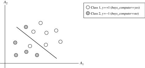
Figure 9.10 A simple 2-D case showing linearly inseparable data. Unlike the linear separable data of Figure 9.7, here it is not possible to draw a straight line to separate the classes. Instead, the decision boundary is nonlinear.
The good news is that the approach described for linear SVMs can be extended to create nonlinear SVMs for the classification of linearly inseparable data (also called nonlinearly separable data, or nonlinear data for short). Such SVMs are capable of finding nonlinear decision boundaries (i.e., nonlinear hypersurfaces) in input space.
“So,” you may ask, “how can we extend the linear approach?” We obtain a nonlinear SVM by extending the approach for linear SVMs as follows. There are two main steps. In the first step, we transform the original input data into a higher dimensional space using a nonlinear mapping. Several common nonlinear mappings can be used in this step, as we will further describe next. Once the data have been transformed into the new higher space, the second step searches for a linear separating hyperplane in the new space. We again end up with a quadratic optimization problem that can be solved using the linear SVM formulation. The maximal marginal hyperplane found in the new space corresponds to a nonlinear separating hypersurface in the original space.
Example 9.2
Nonlinear transformation of original input data into a higher dimensional space
Consider the following example. A 3-D input vector ![]() is mapped into a 6-D space, Z, using the mappings
is mapped into a 6-D space, Z, using the mappings ![]() ,
, ![]() , and
, and ![]() . A decision hyperplane in the new space is
. A decision hyperplane in the new space is ![]() , where W and Z are vectors. This is linear. We solve for W and b and then substitute back so that the linear decision hyperplane in the new (Z) space corresponds to a nonlinear second-order polynomial in the original 3-D input space:
, where W and Z are vectors. This is linear. We solve for W and b and then substitute back so that the linear decision hyperplane in the new (Z) space corresponds to a nonlinear second-order polynomial in the original 3-D input space:
![]()
But there are some problems. First, how do we choose the nonlinear mapping to a higher dimensional space? Second, the computation involved will be costly. Refer to Eq. (9.19) for the classification of a test tuple, ![]() . Given the test tuple, we have to compute its dot product with every one of the support vectors.3 In training, we have to compute a similar dot product several times in order to find the MMH. This is especially expensive. Hence, the dot product computation required is very heavy and costly. We need another trick!
. Given the test tuple, we have to compute its dot product with every one of the support vectors.3 In training, we have to compute a similar dot product several times in order to find the MMH. This is especially expensive. Hence, the dot product computation required is very heavy and costly. We need another trick!
Luckily, we can use another math trick. It so happens that in solving the quadratic optimization problem of the linear SVM (i.e., when searching for a linear SVM in the new higher dimensional space), the training tuples appear only in the form of dot products, ![]() , where
, where ![]() is simply the nonlinear mapping function applied to transform the training tuples. Instead of computing the dot product on the transformed data tuples, it turns out that it is mathematically equivalent to instead apply a kernel function,
is simply the nonlinear mapping function applied to transform the training tuples. Instead of computing the dot product on the transformed data tuples, it turns out that it is mathematically equivalent to instead apply a kernel function, ![]() , to the original input data. That is,
, to the original input data. That is,
![]() (9.20)
(9.20)
In other words, everywhere that ![]() appears in the training algorithm, we can replace it with
appears in the training algorithm, we can replace it with ![]() . In this way, all calculations are made in the original input space, which is of potentially much lower dimensionality! We can safely avoid the mapping—it turns out that we don’t even have to know what the mapping is! We will talk more later about what kinds of functions can be used as kernel functions for this problem.
. In this way, all calculations are made in the original input space, which is of potentially much lower dimensionality! We can safely avoid the mapping—it turns out that we don’t even have to know what the mapping is! We will talk more later about what kinds of functions can be used as kernel functions for this problem.
After applying this trick, we can then proceed to find a maximal separating hyperplane. The procedure is similar to that described in Section 9.3.1, although it involves placing a user-specified upper bound, C, on the Lagrange multipliers, ![]() . This upper bound is best determined experimentally.
. This upper bound is best determined experimentally.
“What are some of the kernel functions that could be used?” Properties of the kinds of kernel functions that could be used to replace the dot product scenario just described have been studied. Three admissible kernel functions are
Each of these results in a different nonlinear classifier in (the original) input space. Neural network aficionados will be interested to note that the resulting decision hyperplanes found for nonlinear SVMs are the same type as those found by other well-known neural network classifiers. For instance, an SVM with a Gaussian radial basis function (RBF) gives the same decision hyperplane as a type of neural network known as a radial basis function network. An SVM with a sigmoid kernel is equivalent to a simple two-layer neural network known as a multilayer perceptron (with no hidden layers).
There are no golden rules for determining which admissible kernel will result in the most accurate SVM. In practice, the kernel chosen does not generally make a large difference in resulting accuracy. SVM training always finds a global solution, unlike neural networks, such as backpropagation, where many local minima usually exist (Section 9.2.3).
So far, we have described linear and nonlinear SVMs for binary (i.e., two-class) classification. SVM classifiers can be combined for the multiclass case. See Section 9.7.1 for some strategies, such as training one classifier per class and the use of error-correcting codes.
A major research goal regarding SVMs is to improve the speed in training and testing so that SVMs may become a more feasible option for very large data sets (e.g., millions of support vectors). Other issues include determining the best kernel for a given data set and finding more efficient methods for the multiclass case.