
11.3 Clustering Graph and Network Data
Cluster analysis on graph and network data extracts valuable knowledge and information. Such data are increasingly popular in many applications. We discuss applications and challenges of clustering graph and network data in Section 11.3.1. Similarity measures for this form of clustering are given in Section 11.3.2. You will learn about graph clustering methods in Section 11.3.3.
In general, the terms graph and network can be used interchangeably. In the rest of this section, we mainly use the term graph.
11.3.1 Applications and Challenges
As a customer relationship manager at AllElectronics, you notice that a lot of data relating to customers and their purchase behavior can be preferably modeled using graphs.
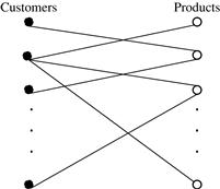
Bipartite graphs are widely used in many applications. Consider another example.
In addition to bipartite graphs, cluster analysis can also be applied to other types of graphs, including general graphs, as elaborated Example 11.18.
“Are there any challenges specific to cluster analysis on graph and network data?” In most of the clustering methods discussed so far, objects are represented using a set of attributes. A unique feature of graph and network data is that only objects (as vertices) and relationships between them (as edges) are given. No dimensions or attributes are explicitly defined. To conduct cluster analysis on graph and network data, there are two major new challenges.
■ “How can we measure the similarity between two objects on a graph accordingly?” Typically, we cannot use conventional distance measures, such as Euclidean distance. Instead, we need to develop new measures to quantify the similarity. Such measures often are not metric, and thus raise new challenges regarding the development of efficient clustering methods. Similarity measures for graphs are discussed in Section 11.3.2.
■ “How can we design clustering models and methods that are effective on graph and network data?” Graph and network data are often complicated, carrying topological structures that are more sophisticated than traditional cluster analysis applications. Many graph data sets are large, such as the web graph containing at least tens of billions of web pages in the publicly indexable Web. Graphs can also be sparse where, on average, a vertex is connected to only a small number of other vertices in the graph. To discover accurate and useful knowledge hidden deep in the data, a good clustering method has to accommodate these factors. Clustering methods for graph and network data are introduced in Section 11.3.3.
11.3.2 Similarity Measures
“How can we measure the similarity or distance between two vertices in a graph?” In our discussion, we examine two types of measures: geodesic distance and distance based on random walk.
Geodesic Distance
A simple measure of the distance between two vertices in a graph is the shortest path between the vertices. Formally, the geodesic distance between two vertices is the length in terms of the number of edges of the shortest path between the vertices. For two vertices that are not connected in a graph, the geodesic distance is defined as infinite.
Using geodesic distance, we can define several other useful measurements for graph analysis and clustering. Given a graph ![]() , where V is the set of vertices and E is the set of edges, we define the following:
, where V is the set of vertices and E is the set of edges, we define the following:
■ For a vertext ![]() , the eccentricity of v, denoted
, the eccentricity of v, denoted ![]() , is the largest geodesic distance between v and any other vertex
, is the largest geodesic distance between v and any other vertex ![]() . The eccentricity of v captures how far away v is from its remotest vertex in the graph.
. The eccentricity of v captures how far away v is from its remotest vertex in the graph.
■ The radius of graph G is the minimum eccentricity of all vertices. That is,
![]() (11.27)
(11.27)
The radius captures the distance between the “most central point” and the “farthest border” of the graph.
■ The diameter of graph G is the maximum eccentricity of all vertices. That is,
![]() (11.28)
(11.28)
The diameter represents the largest distance between any pair of vertices.
■ A peripheral vertex is a vertex that achieves the diameter.
Example 11.19
Measurements based on geodesic distance
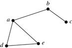
Consider graph G in Figure 11.13. The eccentricity of a is 2, that is, ![]() ,
, ![]() , and
, and ![]() . Thus, the radius of G is 2, and the diameter is 3. Note that it is not necessary that
. Thus, the radius of G is 2, and the diameter is 3. Note that it is not necessary that ![]() . Vertices c, d, and e are peripheral vertices.
. Vertices c, d, and e are peripheral vertices.
SimRank: Similarity Based on Random Walk and Structural Context
For some applications, geodesic distance may be inappropriate in measuring the similarity between vertices in a graph. Here we introduce SimRank, a similarity measure based on random walk and on the structural context of the graph. In mathematics, a random walk is a trajectory that consists of taking successive random steps.
Let’s have a closer look at what is meant by similarity based on structural context, and similarity based on random walk.
The intuition behind similarity based on structural context is that two vertices in a graph are similar if they are connected to similar vertices. To measure such similarity, we need to define the notion of individual neighborhood. In a directed graph ![]() , where V is the set of vertices and
, where V is the set of vertices and ![]() is the set of edges, for a vertex
is the set of edges, for a vertex ![]() , the individual in-neighborhood of v is defined as
, the individual in-neighborhood of v is defined as
![]() (11.29)
(11.29)
Symmetrically, we define the individual out-neighborhood of v as
![]() (11.30)
(11.30)
Following the intuition illustrated in Example 11.20, we define SimRank, a structural-context similarity, with a value that is between 0 and 1 for any pair of vertices. For any vertex, ![]() , the similarity between the vertex and itself is
, the similarity between the vertex and itself is ![]() because the neighborhoods are identical. For vertices
because the neighborhoods are identical. For vertices ![]() such that
such that ![]() , we can define
, we can define
![]() (11.31)
(11.31)
where C is a constant between 0 and 1. A vertex may not have any in-neighbors. Thus, we define Eq. (11.31) to be 0 when either I(u) or I(v) is ∅. Parameter C specifies the rate of decay as similarity is propagated across edges.
“How can we compute SimRank?” A straightforward method iteratively evaluates Eq. (11.31) until a fixed point is reached. Let ![]() be the SimRank score calculated at the i th round. To begin, we set
be the SimRank score calculated at the i th round. To begin, we set
![]() (11.32)
(11.32)
We use Eq. (11.31) to compute ![]() from si as
from si as
![]() (11.33)
(11.33)
It can be shown that ![]() . Additional methods for approximating SimRank are given in the bibliographic notes (Section 11.7).
. Additional methods for approximating SimRank are given in the bibliographic notes (Section 11.7).
Now, let’s consider similarity based on random walk. A directed graph is strongly connected if, for any two nodes u and v, there is a path from u to v and another path from v to u. In a strongly connected graph, ![]() , for any two vertices,
, for any two vertices, ![]() , we can define the expected distance from u to v as
, we can define the expected distance from u to v as
![]() (11.34)
(11.34)
where ![]() is a path starting from u and ending at v that may contain cycles but does not reach v until the end. For a traveling tour,
is a path starting from u and ending at v that may contain cycles but does not reach v until the end. For a traveling tour, ![]() , its length is
, its length is ![]() . The probability of the tour is defined as
. The probability of the tour is defined as
 (11.35)
To measure the probability that a vertex w receives a message that originated simultaneously from u and v, we extend the expected distance to the notion of expected meeting distance, that is,
![]() (11.36)
(11.36)
where ![]() is a pair of tours
is a pair of tours ![]() and
and ![]() of the same length. Using a constant C between 0 and 1, we define the expected meeting probability as
of the same length. Using a constant C between 0 and 1, we define the expected meeting probability as
![]() (11.37)
(11.37)
which is a similarity measure based on random walk. Here, the parameter C specifies the probability of continuing the walk at each step of the trajectory.
It has been shown that ![]() for any two vertices, u and v. That is, SimRank is based on both structural context and random walk.
for any two vertices, u and v. That is, SimRank is based on both structural context and random walk.
11.3.3 Graph Clustering Methods
Let’s consider how to conduct clustering on a graph. We first describe the intuition behind graph clustering. We then discuss two general categories of graph clustering methods.
To find clusters in a graph, imagine cutting the graph into pieces, each piece being a cluster, such that the vertices within a cluster are well connected and the vertices in different clusters are connected in a much weaker way. Formally, for a graph, ![]() , a cut,
, a cut, ![]() , is a partitioning of the set of vertices V in G, that is,
, is a partitioning of the set of vertices V in G, that is, ![]() and
and ![]() . The cut set of a cut is the set of edges,
. The cut set of a cut is the set of edges, ![]() . The size of the cut is the number of edges in the cut set. For weighted graphs, the size of a cut is the sum of the weights of the edges in the cut set.
. The size of the cut is the number of edges in the cut set. For weighted graphs, the size of a cut is the sum of the weights of the edges in the cut set.
“What kinds of cuts are good for deriving clusters in graphs?” In graph theory and some network applications, a minimum cut is of importance. A cut is minimum if the cut’s size is not greater than any other cut’s size. There are polynomial time algorithms to compute minimum cuts of graphs. Can we use these algorithms in graph clustering?
Example 11.21
Cuts and clusters
Consider graph G in Figure 11.14. The graph has two clusters: ![]() and
and ![]() , and one outlier vertex, l.
, and one outlier vertex, l.
Consider cut ![]() . Only one edge, namely, (e, l), crosses the two partitions created by C1. Therefore, the cut set of C1 is
. Only one edge, namely, (e, l), crosses the two partitions created by C1. Therefore, the cut set of C1 is ![]() and the size of C1 is 1. (Note that the size of any cut in a connected graph cannot be smaller than 1.) As a minimum cut, C1 does not lead to a good clustering because it only separates the outlier vertex, l, from the rest of the graph.
and the size of C1 is 1. (Note that the size of any cut in a connected graph cannot be smaller than 1.) As a minimum cut, C1 does not lead to a good clustering because it only separates the outlier vertex, l, from the rest of the graph.
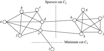
Cut ![]() leads to a much better clustering than C1.
leads to a much better clustering than C1.
The edges in the cut set of C2 are those connecting the two “natural clusters” in the graph. Specifically, for edges (d, h) and (e, k) that are in the cut set, most of the edges connecting d, h, e, and k belong to one cluster.
Example 11.21 indicates that using a minimum cut is unlikely to lead to a good clustering. We are better off choosing a cut where, for each vertex u that is involved in an edge in the cut set, most of the edges connecting to u belong to one cluster. Formally, let ![]() be the degree of u, that is, the number of edges connecting to u. The sparsity of a cut
be the degree of u, that is, the number of edges connecting to u. The sparsity of a cut ![]() is defined as
is defined as
![]() (11.38)
(11.38)
A cut is sparsest if its sparsity is not greater than the sparsity of any other cut. There may be more than one sparsest cut.
In Example 11.21 and Figure 11.14, C2 is a sparsest cut. Using sparsity as the objective function, a sparsest cut tries to minimize the number of edges crossing the partitions and balance the partitions in size.
Consider a clustering on a graph ![]() that partitions the graph into k clusters. The modularity of a clustering assesses the quality of the clustering and is defined as
that partitions the graph into k clusters. The modularity of a clustering assesses the quality of the clustering and is defined as
![]() (11.39)
(11.39)
where li is the number of edges between vertices in the i th cluster, and di is the sum of the degrees of the vertices in the i th cluster. The modularity of a clustering of a graph is the difference between the fraction of all edges that fall into individual clusters and the fraction that would do so if the graph vertices were randomly connected. The optimal clustering of graphs maximizes the modularity.
Theoretically, many graph clustering problems can be regarded as finding good cuts, such as the sparsest cuts, on the graph. In practice, however, a number of challenges exist:
■ High computational cost: Many graph cut problems are computationally expensive. The sparsest cut problem, for example, is NP-hard. Therefore, finding the optimal solutions on large graphs is often impossible. A good trade-off between efficiency/scalability and quality has to be achieved.
■ Sophisticated graphs: Graphs can be more sophisticated than the ones described here, involving weights and/or cycles.
■ High dimensionality: A graph can have many vertices. In a similarity matrix, a vertex is represented as a vector (a row in the matrix) with a dimensionality that is the number of vertices in the graph. Therefore, graph clustering methods must handle high dimensionality.
■ Sparsity: A large graph is often sparse, meaning each vertex on average connects to only a small number of other vertices. A similarity matrix from a large sparse graph can also be sparse.
There are two kinds of methods for clustering graph data, which address these challenges. One uses clustering methods for high-dimensional data, while the other is designed specifically for clustering graphs.
The first group of methods is based on generic clustering methods for high-dimensional data. They extract a similarity matrix from a graph using a similarity measure such as those discussed in Section 11.3.2. A generic clustering method can then be applied on the similarity matrix to discover clusters. Clustering methods for high-dimensional data are typically employed. For example, in many scenarios, once a similarity matrix is obtained, spectral clustering methods (Section 11.2.4) can be applied. Spectral clustering can approximate optimal graph cut solutions. For additional information, please refer to the bibliographic notes (Section 11.7).
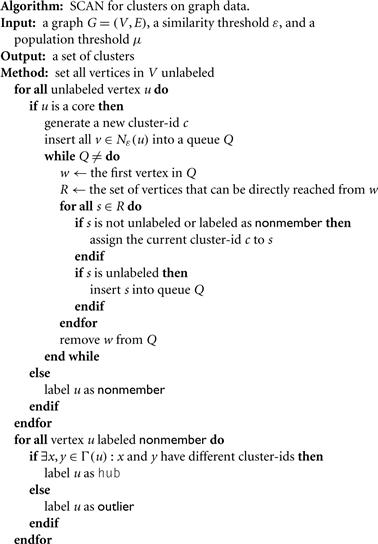
The second group of methods is specific to graphs. They search the graph to find well-connected components as clusters. Let’s look at a method called SCAN (Structural Clustering Algorithm for Networks) as an example.
Given an undirected graph, ![]() , for a vertex,
, for a vertex, ![]() , the neighborhood of u is
, the neighborhood of u is ![]() . Using the idea of structural-context similarity, SCAN measures the similarity between two vertices,
. Using the idea of structural-context similarity, SCAN measures the similarity between two vertices, ![]() , by the normalized common neighborhood size, that is,
, by the normalized common neighborhood size, that is,
![]() (11.40)
(11.40)
The larger the value computed, the more similar the two vertices. SCAN uses a similarity threshold ε to define the cluster membership. For a vertex, ![]() , the ε-neighborhood of u is defined as
, the ε-neighborhood of u is defined as ![]() . The ε-neighborhood of u contains all neighbors of u with a structural-context similarity to u that is at least ε.
. The ε-neighborhood of u contains all neighbors of u with a structural-context similarity to u that is at least ε.
In SCAN, a core vertex is a vertex inside of a cluster. That is, ![]() is a core vertex if
is a core vertex if ![]() , where μ is a popularity threshold. SCAN grows clusters from core vertices. If a vertex v is in the ε-neighborhood of a core u, then v is assigned to the same cluster as u. This process of growing clusters continues until no cluster can be further grown. The process is similar to the density-based clustering method, DBSCAN (Chapter 10).
, where μ is a popularity threshold. SCAN grows clusters from core vertices. If a vertex v is in the ε-neighborhood of a core u, then v is assigned to the same cluster as u. This process of growing clusters continues until no cluster can be further grown. The process is similar to the density-based clustering method, DBSCAN (Chapter 10).
Formally, a vertex v can be directly reached from a core u if ![]() . Transitively, a vertex v can be reached from a core u if there exist vertices
. Transitively, a vertex v can be reached from a core u if there exist vertices ![]() such that w1 can be reached from u, wi can be reached from
such that w1 can be reached from u, wi can be reached from ![]() for
for ![]() , and v can be reached from wn. Moreover, two vertices,
, and v can be reached from wn. Moreover, two vertices, ![]() , which may or may not be cores, are said to be connected if there exists a core w such that both u and v can be reached from w. All vertices in a cluster are connected. A cluster is a maximum set of vertices such that every pair in the set is connected.
, which may or may not be cores, are said to be connected if there exists a core w such that both u and v can be reached from w. All vertices in a cluster are connected. A cluster is a maximum set of vertices such that every pair in the set is connected.
Some vertices may not belong to any cluster. Such a vertex u is a hub if the neighborhood ![]() of u contains vertices from more than one cluster. If a vertex does not belong to any cluster, and is not a hub, it is an outlier.
of u contains vertices from more than one cluster. If a vertex does not belong to any cluster, and is not a hub, it is an outlier.
The SCAN algorithm is shown in Figure 11.15. The search framework closely resembles the cluster-finding process in DBSCAN. SCAN finds a cut of the graph, where each cluster is a set of vertices that are connected based on the transitive similarity in a structural context.
An advantage of SCAN is that its time complexity is linear with respect to the number of edges. In very large and sparse graphs, the number of edges is in the same scale of the number of vertices. Therefore, SCAN is expected to have good scalability on clustering large graphs.