
8.6 Techniques to Improve Classification Accuracy
In this section, you will learn some tricks for increasing classification accuracy. We focus on ensemble methods. An ensemble for classification is a composite model, made up of a combination of classifiers. The individual classifiers vote, and a class label prediction is returned by the ensemble based on the collection of votes. Ensembles tend to be more accurate than their component classifiers. We start off in Section 8.6.1 by introducing ensemble methods in general. Bagging (Section 8.6.2), boosting (Section 8.6.3), and random forests (Section 8.6.4) are popular ensemble methods.
Traditional learning models assume that the data classes are well distributed. In many real-world data domains, however, the data are class-imbalanced, where the main class of interest is represented by only a few tuples. This is known as the class imbalance problem. We also study techniques for improving the classification accuracy of class-imbalanced data. These are presented in Section 8.6.5.
8.6.1 Introducing Ensemble Methods
Bagging, boosting, and random forests are examples of ensemble methods (Figure 8.21). An ensemble combines a series of k learned models (or base classifiers), ![]() , with the aim of creating an improved composite classification model,
, with the aim of creating an improved composite classification model, ![]() . A given data set, D, is used to create k training sets,
. A given data set, D, is used to create k training sets, ![]() , where
, where ![]() is used to generate classifier Mi. Given a new data tuple to classify, the base classifiers each vote by returning a class prediction. The ensemble returns a class prediction based on the votes of the base classifiers.
is used to generate classifier Mi. Given a new data tuple to classify, the base classifiers each vote by returning a class prediction. The ensemble returns a class prediction based on the votes of the base classifiers.

Figure 8.21 Increasing classifier accuracy: Ensemble methods generate a set of classification models, M1, M2, …, Mk. Given a new data tuple to classify, each classifier “votes” for the class label of that tuple. The ensemble combines the votes to return a class prediction.
An ensemble tends to be more accurate than its base classifiers. For example, consider an ensemble that performs majority voting. That is, given a tuple X to classify, it collects the class label predictions returned from the base classifiers and outputs the class in majority. The base classifiers may make mistakes, but the ensemble will misclassify X only if over half of the base classifiers are in error. Ensembles yield better results when there is significant diversity among the models. That is, ideally, there is little correlation among classifiers. The classifiers should also perform better than random guessing. Each base classifier can be allocated to a different CPU and so ensemble methods are parallelizable.
To help illustrate the power of an ensemble, consider a simple two-class problem described by two attributes, x1 and x2. The problem has a linear decision boundary. Figure 8.22(a) shows the decision boundary of a decision tree classifier on the problem. Figure 8.22(b) shows the decision boundary of an ensemble of decision tree classifiers on the same problem. Although the ensemble’s decision boundary is still piecewise constant, it has a finer resolution and is better than that of a single tree.
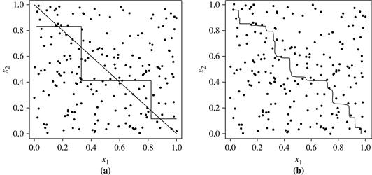
Figure 8.22 Decision boundary by (a) a single decision tree and (b) an ensemble of decision trees for a linearly separable problem (i.e., where the actual decision boundary is a straight line). The decision tree struggles with approximating a linear boundary. The decision boundary of the ensemble is closer to the true boundary. Source: From Seni and Elder [SE10]. Copyright © (2010) Morgan & Claypool Publishers; used with permission.
8.6.2 Bagging
We now take an intuitive look at how bagging works as a method of increasing accuracy. Suppose that you are a patient and would like to have a diagnosis made based on your symptoms. Instead of asking one doctor, you may choose to ask several. If a certain diagnosis occurs more than any other, you may choose this as the final or best diagnosis. That is, the final diagnosis is made based on a majority vote, where each doctor gets an equal vote. Now replace each doctor by a classifier, and you have the basic idea behind bagging. Intuitively, a majority vote made by a large group of doctors may be more reliable than a majority vote made by a small group.
Given a set, D, of D tuples, bagging works as follows. For iteration ![]() , a training set, Di, of D tuples is sampled with replacement from the original set of tuples, D. Note that the term bagging stands for bootstrap aggregation. Each training set is a bootstrap sample, as described in Section 8.5.4. Because sampling with replacement is used, some of the original tuples of D may not be included in Di, whereas others may occur more than once. A classifier model, Mi, is learned for each training set, Di. To classify an unknown tuple, X, each classifier, Mi, returns its class prediction, which counts as one vote. The bagged classifier,
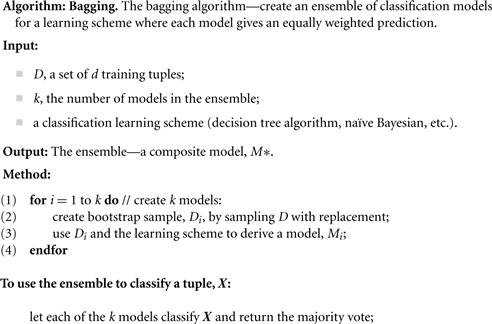
, a training set, Di, of D tuples is sampled with replacement from the original set of tuples, D. Note that the term bagging stands for bootstrap aggregation. Each training set is a bootstrap sample, as described in Section 8.5.4. Because sampling with replacement is used, some of the original tuples of D may not be included in Di, whereas others may occur more than once. A classifier model, Mi, is learned for each training set, Di. To classify an unknown tuple, X, each classifier, Mi, returns its class prediction, which counts as one vote. The bagged classifier, ![]() , counts the votes and assigns the class with the most votes to X. Bagging can be applied to the prediction of continuous values by taking the average value of each prediction for a given test tuple. The algorithm is summarized in Figure 8.23.
, counts the votes and assigns the class with the most votes to X. Bagging can be applied to the prediction of continuous values by taking the average value of each prediction for a given test tuple. The algorithm is summarized in Figure 8.23.
The bagged classifier often has significantly greater accuracy than a single classifier derived from D, the original training data. It will not be considerably worse and is more robust to the effects of noisy data and overfitting. The increased accuracy occurs because the composite model reduces the variance of the individual classifiers.
8.6.3 Boosting and AdaBoost
We now look at the ensemble method of boosting. As in the previous section, suppose that as a patient, you have certain symptoms. Instead of consulting one doctor, you choose to consult several. Suppose you assign weights to the value or worth of each doctor’s diagnosis, based on the accuracies of previous diagnoses they have made. The final diagnosis is then a combination of the weighted diagnoses. This is the essence behind boosting.
In boosting, weights are also assigned to each training tuple. A series of k classifiers is iteratively learned. After a classifier, Mi, is learned, the weights are updated to allow the subsequent classifier, ![]() , to “pay more attention” to the training tuples that were misclassified by Mi. The final boosted classifier,
, to “pay more attention” to the training tuples that were misclassified by Mi. The final boosted classifier, ![]() , combines the votes of each individual classifier, where the weight of each classifier’s vote is a function of its accuracy.
, combines the votes of each individual classifier, where the weight of each classifier’s vote is a function of its accuracy.
AdaBoost (short for Adaptive Boosting) is a popular boosting algorithm. Suppose we want to boost the accuracy of a learning method. We are given D, a data set of D class-labeled tuples, ![]() , where yi is the class label of tuple
, where yi is the class label of tuple ![]() . Initially, AdaBoost assigns each training tuple an equal weight of
. Initially, AdaBoost assigns each training tuple an equal weight of ![]() . Generating k classifiers for the ensemble requires k rounds through the rest of the algorithm. We can sample to form any sized training set, not necessarily of size d. Sampling with replacement is used—the same tuple may be selected more than once. Each tuple’s chance of being selected is based on its weight. A classifier model, Mi, is derived from the training tuples of Di. Its error is then calculated using Di as a test set. The weights of the training tuples are then adjusted according to how they were classified.
. Generating k classifiers for the ensemble requires k rounds through the rest of the algorithm. We can sample to form any sized training set, not necessarily of size d. Sampling with replacement is used—the same tuple may be selected more than once. Each tuple’s chance of being selected is based on its weight. A classifier model, Mi, is derived from the training tuples of Di. Its error is then calculated using Di as a test set. The weights of the training tuples are then adjusted according to how they were classified.
If a tuple was incorrectly classified, its weight is increased. If a tuple was correctly classified, its weight is decreased. A tuple’s weight reflects how difficult it is to classify—the higher the weight, the more often it has been misclassified. These weights will be used to generate the training samples for the classifier of the next round. The basic idea is that when we build a classifier, we want it to focus more on the misclassified tuples of the previous round. Some classifiers may be better at classifying some “difficult” tuples than others. In this way, we build a series of classifiers that complement each other. The algorithm is summarized in Figure 8.24.
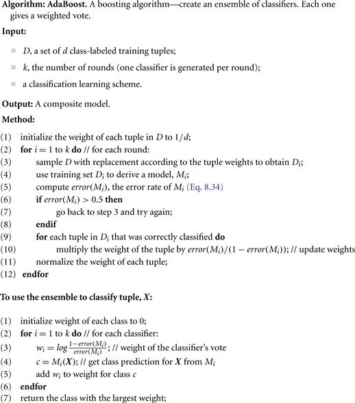
Now, let’s look at some of the math that’s involved in the algorithm. To compute the error rate of model Mi, we sum the weights of each of the tuples in Di that Mi misclassified. That is,
![]() (8.34)
(8.34)
where ![]() is the misclassification error of tuple
is the misclassification error of tuple ![]() : If the tuple was misclassified, then
: If the tuple was misclassified, then ![]() is 1; otherwise, it is 0. If the performance of classifier Mi is so poor that its error exceeds 0.5, then we abandon it. Instead, we try again by generating a new Di training set, from which we derive a new Mi.
is 1; otherwise, it is 0. If the performance of classifier Mi is so poor that its error exceeds 0.5, then we abandon it. Instead, we try again by generating a new Di training set, from which we derive a new Mi.
The error rate of Mi affects how the weights of the training tuples are updated. If a tuple in round i was correctly classified, its weight is multiplied by ![]() . Once the weights of all the correctly classified tuples are updated, the weights for all tuples (including the misclassified ones) are normalized so that their sum remains the same as it was before. To normalize a weight, we multiply it by the sum of the old weights, divided by the sum of the new weights. As a result, the weights of misclassified tuples are increased and the weights of correctly classified tuples are decreased, as described before.
. Once the weights of all the correctly classified tuples are updated, the weights for all tuples (including the misclassified ones) are normalized so that their sum remains the same as it was before. To normalize a weight, we multiply it by the sum of the old weights, divided by the sum of the new weights. As a result, the weights of misclassified tuples are increased and the weights of correctly classified tuples are decreased, as described before.
“Once boosting is complete, how is the ensemble of classifiers used to predict the class label of a tuple, X?” Unlike bagging, where each classifier was assigned an equal vote, boosting assigns a weight to each classifier’s vote, based on how well the classifier performed. The lower a classifier’s error rate, the more accurate it is, and therefore, the higher its weight for voting should be. The weight of classifier Mi’s vote is
![]() (8.35)
(8.35)
For each class, c, we sum the weights of each classifier that assigned class c to X. The class with the highest sum is the “winner” and is returned as the class prediction for tuple X.
“How does boosting compare with bagging?” Because of the way boosting focuses on the misclassified tuples, it risks overfitting the resulting composite model to such data. Therefore, sometimes the resulting “boosted” model may be less accurate than a single model derived from the same data. Bagging is less susceptible to model overfitting. While both can significantly improve accuracy in comparison to a single model, boosting tends to achieve greater accuracy.
8.6.4 Random Forests
We now present another ensemble method called random forests. Imagine that each of the classifiers in the ensemble is a decision tree classifier so that the collection of classifiers is a “forest.” The individual decision trees are generated using a random selection of attributes at each node to determine the split. More formally, each tree depends on the values of a random vector sampled independently and with the same distribution for all trees in the forest. During classification, each tree votes and the most popular class is returned.
Random forests can be built using bagging (Section 8.6.2) in tandem with random attribute selection. A training set, D, of D tuples is given. The general procedure to generate k decision trees for the ensemble is as follows. For each iteration, ![]() ), a training set, Di, of D tuples is sampled with replacement from D. That is, each Di is a bootstrap sample of D (Section 8.5.4), so that some tuples may occur more than once in Di, while others may be excluded. Let F be the number of attributes to be used to determine the split at each node, where F is much smaller than the number of available attributes. To construct a decision tree classifier, Mi, randomly select, at each node, F attributes as candidates for the split at the node. The CART methodology is used to grow the trees. The trees are grown to maximum size and are not pruned. Random forests formed this way, with random input selection, are called Forest-RI.
), a training set, Di, of D tuples is sampled with replacement from D. That is, each Di is a bootstrap sample of D (Section 8.5.4), so that some tuples may occur more than once in Di, while others may be excluded. Let F be the number of attributes to be used to determine the split at each node, where F is much smaller than the number of available attributes. To construct a decision tree classifier, Mi, randomly select, at each node, F attributes as candidates for the split at the node. The CART methodology is used to grow the trees. The trees are grown to maximum size and are not pruned. Random forests formed this way, with random input selection, are called Forest-RI.
Another form of random forest, called Forest-RC, uses random linear combinations of the input attributes. Instead of randomly selecting a subset of the attributes, it creates new attributes (or features) that are a linear combination of the existing attributes. That is, an attribute is generated by specifying L, the number of original attributes to be combined. At a given node, L attributes are randomly selected and added together with coefficients that are uniform random numbers on ![]() . F linear combinations are generated, and a search is made over these for the best split. This form of random forest is useful when there are only a few attributes available, so as to reduce the correlation between individual classifiers.
. F linear combinations are generated, and a search is made over these for the best split. This form of random forest is useful when there are only a few attributes available, so as to reduce the correlation between individual classifiers.
Random forests are comparable in accuracy to AdaBoost, yet are more robust to errors and outliers. The generalization error for a forest converges as long as the number of trees in the forest is large. Thus, overfitting is not a problem. The accuracy of a random forest depends on the strength of the individual classifiers and a measure of the dependence between them. The ideal is to maintain the strength of individual classifiers without increasing their correlation. Random forests are insensitive to the number of attributes selected for consideration at each split. Typically, up to ![]() are chosen. (An interesting empirical observation was that using a single random input attribute may result in good accuracy that is often higher than when using several attributes.) Because random forests consider many fewer attributes for each split, they are efficient on very large databases. They can be faster than either bagging or boosting. Random forests give internal estimates of variable importance.
are chosen. (An interesting empirical observation was that using a single random input attribute may result in good accuracy that is often higher than when using several attributes.) Because random forests consider many fewer attributes for each split, they are efficient on very large databases. They can be faster than either bagging or boosting. Random forests give internal estimates of variable importance.
8.6.5 Improving Classification Accuracy of Class-Imbalanced Data
In this section, we revisit the class imbalance problem. In particular, we study approaches to improving the classification accuracy of class-imbalanced data.
Given two-class data, the data are class-imbalanced if the main class of interest (the positive class) is represented by only a few tuples, while the majority of tuples represent the negative class. For multiclass-imbalanced data, the data distribution of each class differs substantially where, again, the main class or classes of interest are rare. The class imbalance problem is closely related to cost-sensitive learning, wherein the costs of errors, per class, are not equal. In medical diagnosis, for example, it is much more costly to falsely diagnose a cancerous patient as healthy (a false negative) than to misdiagnose a healthy patient as having cancer (a false positive). A false negative error could lead to the loss of life and therefore is much more expensive than a false positive error. Other applications involving class-imbalanced data include fraud detection, the detection of oil spills from satellite radar images, and fault monitoring.
Traditional classification algorithms aim to minimize the number of errors made during classification. They assume that the costs of false positive and false negative errors are equal. By assuming a balanced distribution of classes and equal error costs, they are therefore not suitable for class-imbalanced data. Earlier parts of this chapter presented ways of addressing the class imbalance problem. Although the accuracy measure assumes that the cost of classes are equal, alternative evaluation metrics can be used that consider the different types of classifications. Section 8.5.1, for example, presented sensitivity or recall (the true positive rate) and specificity (the true negative rate), which help to assess how well a classifier can predict the class label of imbalanced data. Additional relevant measures discussed include F1 and ![]() . Section 8.5.6 showed how ROC curves plot sensitivity versus
. Section 8.5.6 showed how ROC curves plot sensitivity versus ![]() (i.e., the false positive rate). Such curves can provide insight when studying the performance of classifiers on class-imbalanced data.
(i.e., the false positive rate). Such curves can provide insight when studying the performance of classifiers on class-imbalanced data.
In this section, we look at general approaches for improving the classification accuracy of class-imbalanced data. These approaches include (1) oversampling, (2) undersampling, (3) threshold moving, and (4) ensemble techniques. The first three do not involve any changes to the construction of the classification model. That is, oversampling and undersampling change the distribution of tuples in the training set; threshold moving affects how the model makes decisions when classifying new data. Ensemble methods follow the techniques described in Sections 8.6.2 through 8.6.4. For ease of explanation, we describe these general approaches with respect to the two-class imbalance data problem, where the higher-cost classes are rarer than the lower-cost classes.
Both oversampling and undersampling change the training data distribution so that the rare (positive) class is well represented. Oversampling works by resampling the positive tuples so that the resulting training set contains an equal number of positive and negative tuples. Undersampling works by decreasing the number of negative tuples. It randomly eliminates tuples from the majority (negative) class until there are an equal number of positive and negative tuples.
Several variations to oversampling and undersampling exist. They may vary, for instance, in how tuples are added or eliminated. For example, the SMOTE algorithm uses oversampling where synthetic tuples are added, which are “close to” the given positive tuples in tuple space.
The threshold-moving approach to the class imbalance problem does not involve any sampling. It applies to classifiers that, given an input tuple, return a continuous output value (just like in Section 8.5.6, where we discussed how to construct ROC curves). That is, for an input tuple, X, such a classifier returns as output a mapping, ![]() . Rather than manipulating the training tuples, this method returns a classification decision based on the output values. In the simplest approach, tuples for which
. Rather than manipulating the training tuples, this method returns a classification decision based on the output values. In the simplest approach, tuples for which ![]() , for some threshold, t, are considered positive, while all other tuples are considered negative. Other approaches may involve manipulating the outputs by weighting. In general, threshold moving moves the threshold, t, so that the rare class tuples are easier to classify (and hence, there is less chance of costly false negative errors). Examples of such classifiers include naïve Bayesian classifiers (Section 8.3) and neural network classifiers like backpropagation (Section 9.2). The threshold-moving method, although not as popular as over- and undersampling, is simple and has shown some success for the two-class-imbalanced data.
, for some threshold, t, are considered positive, while all other tuples are considered negative. Other approaches may involve manipulating the outputs by weighting. In general, threshold moving moves the threshold, t, so that the rare class tuples are easier to classify (and hence, there is less chance of costly false negative errors). Examples of such classifiers include naïve Bayesian classifiers (Section 8.3) and neural network classifiers like backpropagation (Section 9.2). The threshold-moving method, although not as popular as over- and undersampling, is simple and has shown some success for the two-class-imbalanced data.
Ensemble methods (Sections 8.6.2 through 8.6.4) have also been applied to the class imbalance problem. The individual classifiers making up the ensemble may include versions of the approaches described here such as oversampling and threshold moving.
These methods work relatively well for the class imbalance problem on two-class tasks. Threshold-moving and ensemble methods were empirically observed to outperform oversampling and undersampling. Threshold moving works well even on data sets that are extremely imbalanced. The class imbalance problem on multiclass tasks is much more difficult, where oversampling and threshold moving are less effective. Although threshold-moving and ensemble methods show promise, finding a solution for the multiclass imbalance problem remains an area of future work.