6.1.1 Market Basket Analysis: A Motivating Example

Frequent itemset mining leads to the discovery of associations and correlations among items in large transactional or relational data sets. With massive amounts of data continuously being collected and stored, many industries are becoming interested in mining such patterns from their databases. The discovery of interesting correlation relationships among huge amounts of business transaction records can help in many business decision-making processes such as catalog design, cross-marketing, and customer shopping behavior analysis.

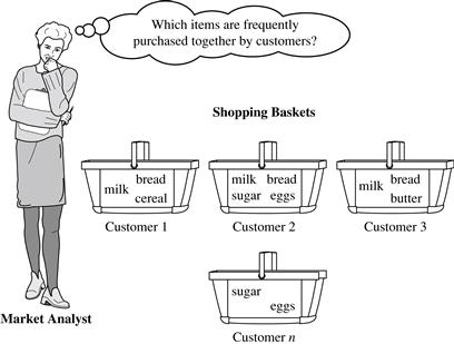
A typical example of frequent itemset mining is market basket analysis. This process analyzes customer buying habits by finding associations between the different items that customers place in their “shopping baskets” (Figure 6.1). The discovery of these associations can help retailers develop marketing strategies by gaining insight into which items are frequently purchased together by customers. For instance, if customers are buying milk, how likely are they to also buy bread (and what kind of bread) on the same trip to the supermarket? This information can lead to increased sales by helping retailers do selective marketing and plan their shelf space.

Let’s look at an example of how market basket analysis can be useful.

If we think of the universe as the set of items available at the store, then each item has a Boolean variable representing the presence or absence of that item. Each basket can then be represented by a Boolean vector of values assigned to these variables. The Boolean vectors can be analyzed for buying patterns that reflect items that are frequently associated or purchased together. These patterns can be represented in the form of association rules. For example, the information that customers who purchase computers also tend to buy antivirus software at the same time is represented in the following association rule:

(6.1)

Rule support and confidence are two measures of rule interestingness. They respectively reflect the usefulness and certainty of discovered rules. A support of 2% for Rule (6.1) means that 2% of all the transactions under analysis show that computer and antivirus software are purchased together. A confidence of 60% means that 60% of the customers who purchased a computer also bought the software. Typically, association rules are considered interesting if they satisfy both a minimum support threshold and a minimum confidence threshold. These thresholds can be a set by users or domain experts. Additional analysis can be performed to discover interesting statistical correlations between associated items.

6.1.2 Frequent Itemsets, Closed Itemsets, and Association Rules

Let be an itemset. Let D, the task-relevant data, be a set of database transactions where each transaction T is a nonempty itemset such that . Each transaction is associated with an identifier, called a TID. Let A be a set of items. A transaction T is said to contain A if . An association rule is an implication of the form , where , , , , and . The rule holds in the transaction set D with support s, where s is the percentage of transactions in D that contain (i.e., the union of sets A and B say, or, both A and B). This is taken to be the probability, .¹ The rule has confidence c in the transaction set D, where c is the percentage of transactions in D containing A that also contain B. This is taken to be the conditional probability, . That is,

(6.2)

(6.3)

Rules that satisfy both a minimum support threshold (min_sup) and a minimum confidence threshold (min_conf) are called strong. By convention, we write support and confidence values so as to occur between 0% and 100%, rather than 0 to 1.0.

A set of items is referred to as an itemset.² An itemset that contains k items is a k-itemset. The set {computer, antivirus_software } is a 2-itemset. The occurrence frequency of an itemset is the number of transactions that contain the itemset. This is also known, simply, as the frequency, support count, or count of the itemset. Note that the itemset support defined in Eq. (6.2) is sometimes referred to as relative support, whereas the occurrence frequency is called the absolute support. If the relative support of an itemset I satisfies a prespecified minimum support threshold (i.e., the absolute support of I satisfies the corresponding minimum support count threshold), then I is a frequent itemset.³ The set of frequent k-itemsets is commonly denoted by L_k.⁴

From Eq. (6.3), we have

(6.4)

Equation (6.4) shows that the confidence of rule can be easily derived from the support counts of A and . That is, once the support counts of A, B, and are found, it is straightforward to derive the corresponding association rules and and check whether they are strong. Thus, the problem of mining association rules can be reduced to that of mining frequent itemsets.

In general, association rule mining can be viewed as a two-step process:

Additional interestingness measures can be applied for the discovery of correlation relationships between associated items, as will be discussed in Section 6.3. Because the second step is much less costly than the first, the overall performance of mining association rules is determined by the first step.

A major challenge in mining frequent itemsets from a large data set is the fact that such mining often generates a huge number of itemsets satisfying the minimum support (min_sup) threshold, especially when min_sup is set low. This is because if an itemset is frequent, each of its subsets is frequent as well. A long itemset will contain a combinatorial number of shorter, frequent sub-itemsets. For example, a frequent itemset of length 100, such as {}, contains frequent 1-itemsets: , , …, ; frequent 2-itemsets: , ,…,; and so on. The total number of frequent itemsets that it contains is thus

(6.5)

This is too huge a number of itemsets for any computer to compute or store. To overcome this difficulty, we introduce the concepts of closed frequent itemset and maximal frequent itemset.

An itemset X is closed in a data set D if there exists no proper super-itemset Y⁵ such that Y has the same support count as X in D. An itemset X is a closed frequent itemset in set D if X is both closed and frequent in D. An itemset X is a maximal frequent itemset (or max-itemset) in a data set D if X is frequent, and there exists no super-itemset Y such that and Y is frequent in D.

Let be the set of closed frequent itemsets for a data set D satisfying a minimum support threshold, . Let be the set of maximal frequent itemsets for D satisfying . Suppose that we have the support count of each itemset in and . Notice that and its count information can be used to derive the whole set of frequent itemsets. Thus, we say that contains complete information regarding its corresponding frequent itemsets. On the other hand, registers only the support of the maximal itemsets. It usually does not contain the complete support information regarding its corresponding frequent itemsets. We illustrate these concepts with Example 6.2.